Machine Learning

 

CHAITANYA (Deemed to be) University

BTech - III Yr/V Semester CSE

PCC CS-504 -- MACHINE LEARNING

DEPARTMENT OF COMPUTER SCIENCE & ENGINEERING (AI & DS/ML)

 

Course Objective: The students will understand the basics of Machine Learning. They will also learn and will be able to apply different machine learning models to various datasets.

 

 

UNIT-I: INTRODUCTION  

Review of Linear Algebra, Definition of learning systems, Designing a learning system, Classification of learning system, Basic concepts in Machine Learning, Goals and applications of machine learning,  Real life examples of Machine Learning, Regression, Linear Regression, Multivariate Regression.

 

 

UNIT-II: MACHINE LEARNING APPLICATIONS

Decision Tree Learning, representation and Algorithm, appropriate problems for decision tree learning, hypothesis space search decision tree learning, Inductive bias in decision tree learning, issues in decision tree learning, Probabilistic generative model – Naive Bayes, Maximum margin classifier.

 

 

UNIT-III: SUPERVISED LEARNING

Supervised learning Classification and Regression: K-Nearest Neighbor, Linear Regression- Bayesian linear regression, gradient descent, Logistic Regression, Support Vector Machine (SVM), Decision Tree, Random Forests, Evaluation Measures: SSE, MME, R2, confusion matrix, precision, recall, F-Score, ROC-Curve

 

 

UNIT-IV: ENSEMBLE & UNSUPERVISED LEARNING

Unsupervised learning, Introduction to clustering, Types of Clustering: Hierarchical, Agglomerative Clustering and Divisive clustering; Partitional Clustering - K-means clustering, Combining multiple learners: Model combination schemes, Voting, Ensemble Learning - bagging, boosting, stacking, Gaussian Mixture Models,

Introduction to Deep Learning, Natural Language Processing, Computer Vision

Artificial Neural Networks, appropriate problems for neural network learning, perception, Back-propagation algorithm.

 

 

 

 

 

Text Books:

1. Introduction to Machine Learning, By Jeeva Jose, Khanna Book Publishing Co., 2020.

2. Machine Learning, By Rajeev Chopra, Khanna Book Publishing Co., 2021.

3. Machine Learning: The New AI, By Ethem Alpaydin, The MIT Press, 2016.

 

References:

1. Ethem Apaydin, Introduction to Machine Learning, 2e. The MIT Press, 2010.

2. Kevin P. Murphy, Machine Learning: a Probabilistic Perspective, The MIT Press, 2012.

3. Tom Mitchell, Machine Learning, McGraw Hill, 1997.

4. Machine Learning: An Algorithmic Perspective, Stephen Marshald, Taylor & Fransis.

 

 

 GIT HUB projects

 

SCAN this QR code to connect with git hub projects

 Ad

 

 

 

 

 

 

 

 

 

 

 

 

 

 

 

 

 

 

 

 

 

 

 

 

 

Linear Algebra for Machine learning

Machine learning has a strong connection with mathematics. Each machine learning algorithm is based on the concepts of mathematics & also with the help of mathematics, one can choose the correct algorithm by considering training time, complexity, number of features, etc. Linear Algebra is an essential field of mathematics, which defines the study of vectors, matrices, planes, mapping, and lines required for linear transformation.

The term Linear Algebra was initially introduced in the early 18^th century to find out the unknowns in Linear equations and solve the equation easily; hence it is an important branch of mathematics that helps study data. Also, no one can deny that Linear Algebra is undoubtedly the important and primary thing to process the applications of Machine Learning. It is also a prerequisite to start learning Machine Learning and data science.

Linear algebra plays a vital role and key foundation in machine learning, and it enables ML algorithms to run on a huge number of datasets.

The concepts of linear algebra are widely used in developing algorithms in machine learning. Although it is used almost in each concept of Machine learning, specifically, it can perform the following task:

Optimization of data.

Applicable in loss functions, regularisation, covariance matrices, Singular Value Decomposition (SVD), Matrix Operations, and support vector machine classification.

Implementation of Linear Regression in Machine Learning.

Besides the above uses, linear algebra is also used in neural networks and the data science field.

Basic mathematics principles and concepts like Linear algebra are the foundation of Machine Learning and Deep Learning systems. To learn and understand Machine Learning or Data Science, one needs to be familiar with linear algebra and optimization theory. In this topic, we will explain all the Linear algebra concepts required for machine learning.

Note: Although linear algebra is a must-know part of mathematics for machine learning, it is not required to get intimate in this. It means it is not required to be an expert in linear algebra; instead, only good knowledge of these concepts is more than enough for machine learning.

Why learn Linear Algebra before learning Machine Learning?

Linear Algebra is just similar to the flour of bakery in Machine Learning. As the cake is based on flour similarly, every Machine Learning Model is also based on Linear Algebra. Further, the cake also needs more ingredients like egg, sugar, cream, soda. Similarly, Machine Learning also requires more concepts as vector calculus, probability, and optimization theory. So, we can say that Machine Learning creates a useful model with the help of the above-mentioned mathematical concepts.

Below are some benefits of learning Linear Algebra before Machine learning:

Better Graphic experience

Improved Statistics

Creating better Machine Learning algorithms

Estimating the forecast of Machine Learning

Easy to Learn

Better Graphics Experience:

Linear Algebra helps to provide better graphical processing in Machine Learning like Image, audio, video, and edge detection. These are the various graphical representations supported by Machine Learning projects that you can work on. Further, parts of the given data set are trained based on their categories by classifiers provided by machine learning algorithms. These classifiers also remove the errors from the trained data.

Moreover, Linear Algebra helps solve and compute large and complex data set through a specific terminology named Matrix Decomposition Techniques. There are two most popular matrix decomposition techniques, which are as follows:

Q-R

L-U

Improved Statistics:

Statistics is an important concept to organize and integrate data in Machine Learning. Also, linear Algebra helps to understand the concept of statistics in a better manner. Advanced statistical topics can be integrated using methods, operations, and notations of linear algebra.

Creating better Machine Learning algorithms:

Linear Algebra also helps to create better supervised as well as unsupervised Machine Learning algorithms.

Few supervised learning algorithms can be created using Linear Algebra, which is as follows:

Logistic Regression

Linear Regression

Decision Trees

Support Vector Machines (SVM)

Further, below are some unsupervised learning algorithms listed that can also be created with the help of linear algebra as follows:

Single Value Decomposition (SVD)

Clustering

Components Analysis

With the help of Linear Algebra concepts, you can also self-customize the various parameters in the live project and understand in-depth knowledge to deliver the same with more accuracy and precision.

Estimating the forecast of Machine Learning:

If you are working on a Machine Learning project, then you must be a broad-minded person and also, you will be able to impart more perspectives. Hence, in this regard, you must increase the awareness and affinity of Machine Learning concepts. You can begin with setting up different graphs, visualization, using various parameters for diverse machine learning algorithms or taking up things that others around you might find difficult to understand.

Easy to Learn:

Linear Algebra is an important department of Mathematics that is easy to understand. It is taken into consideration whenever there is a requirement of advanced mathematics and its applications.

Minimum Linear Algebra for Machine Learning

Notation:

Notation in linear algebra enables you to read algorithm descriptions in papers, books, and websites to understand the algorithm's working. Even if you use for-loops rather than matrix operations, you will be able to piece things together.

Operations:

Working with an advanced level of abstractions in vectors and matrices can make concepts clearer, and it can also help in the description, coding, and even thinking capability. In linear algebra, it is required to learn the basic operations such as addition, multiplication, inversion, transposing of matrices, vectors, etc.

Matrix Factorization:

One of the most recommended areas of linear algebra is matrix factorization, specifically matrix deposition methods such as SVD and QR.

Examples of Linear Algebra in Machine Learning

Below are some popular examples of linear algebra in Machine learning:

Datasets and Data Files

Linear Regression

Recommender Systems

One-hot encoding

Regularization

Principal Component Analysis

Images and Photographs

Singular-Value Decomposition

Deep Learning

Latent Semantic Analysis

Design a Learning System in Machine Learning

 

According to Arthur Samuel “Machine Learning enables a Machine to Automatically learn from Data, Improve performance from an Experience and predict things without explicitly programmed.” In Simple Words, When we fed the Training Data to Machine Learning Algorithm, this algorithm will produce a mathematical model and with the help of the mathematical model, the machine will make a prediction and take a decision without being explicitly programmed. Also, during training data, the more machine will work with it the more it will get experience and the more efficient result is produced. 

 

Example :  In Driverless Car, the training data is fed to Algorithm like how to Drive Car in Highway, Busy and Narrow Street with factors like speed limit, parking, stop at signal etc. After that, a Logical and Mathematical model is created on the basis of that and after that, the car will work according to the logical model. Also, the more data the data is fed the more efficient output is produced.

Designing a Learning System in Machine Learning :

According to Tom Mitchell, “A computer program is said to be learning from experience (E), with respect to some task (T). Thus, the performance measure (P) is the performance at task T, which is measured by P, and it improves with experience E.”

Example: In Spam E-Mail detection,

·         Task, T: To classify mails into Spam or Not Spam.

·         Performance measure, P: Total percent of mails being correctly classified as being “Spam” or “Not Spam”.

·         Experience, E: Set of Mails with label “Spam”

Steps for Designing Learning System are:

 

Step 1) Choosing the Training Experience: The very important and first task is to choose the training data or training experience which will be fed to the Machine Learning Algorithm. It is important to note that the data or experience that we fed to the algorithm must have a significant impact on the Success or Failure of the Model. So Training data or experience should be chosen wisely.

Below are the attributes which will impact on Success and Failure of Data:

·         The training experience will be able to provide direct or indirect feedback regarding choices. For example: While Playing chess the training data will provide feedback to itself like instead of this move if this is chosen the chances of success increases.

·         Second important attribute is the degree to which the learner will control the sequences of training examples. For example: when training data is fed to the machine then at that time accuracy is very less but when it gains experience while playing again and again with itself or opponent the machine algorithm will get feedback and control the chess game accordingly.

·         Third important attribute is how it will represent the distribution of examples over which performance will be measured. For example, a Machine learning algorithm will get experience while going through a number of different cases and different examples. Thus, Machine Learning Algorithm will get more and more experience by passing through more and more examples and hence its performance will increase.

Step 2- Choosing target function: The next important step is choosing the target function. It means according to the knowledge fed to the algorithm the machine learning will choose NextMove function which will describe what type of legal moves should be taken.  For example : While playing chess with the opponent, when opponent will play then the machine learning algorithm will decide what be the number of possible legal moves taken in order to get success.

Step 3- Choosing Representation for Target function: When the machine algorithm will know all the possible legal moves the next step is to choose the optimized move using any representation i.e. using linear Equations, Hierarchical Graph Representation, Tabular form etc. The NextMove function will move the Target move like out of these move which will provide more success rate. For Example : while playing chess machine have 4 possible moves, so the machine will choose that optimized move which will provide success to it.

Step 4- Choosing Function Approximation Algorithm: An optimized move cannot be chosen just with the training data. The training data had to go through with set of example and through these examples the training data will approximates which steps are chosen and after that machine will provide feedback on it. For Example : When a training data of Playing chess is fed  to algorithm so at that time it is not machine algorithm will fail or get success and again from that failure or success it will measure while next move what step should be chosen and what is its success rate.

Step 5- Final Design: The final design is created at last when system goes from number of examples  , failures and success , correct and incorrect decision and what will be the next step etc. Example: DeepBlue is an intelligent  computer which is ML-based won chess game against the chess expert Garry Kasparov, and it became the first computer which had beaten a human chess expert.

 Applications of Machine learning

Machine learning is a buzzword for today's technology, and it is growing very rapidly day by day. We are using machine learning in our daily life even without knowing it such as Google Maps, Google assistant, Alexa, etc. Below are some most trending real-world applications of Machine Learning:

1. Image Recognition:

Image recognition is one of the most common applications of machine learning. It is used to identify objects, persons, places, digital images, etc. The popular use case of image recognition and face detection is, Automatic friend tagging suggestion:

Facebook provides us a feature of auto friend tagging suggestion. Whenever we upload a photo with our Facebook friends, then we automatically get a tagging suggestion with name, and the technology behind this is machine learning's face detection and recognition algorithm.

It is based on the Facebook project named "Deep Face," which is responsible for face recognition and person identification in the picture.

2. Speech Recognition

While using Google, we get an option of "Search by voice," it comes under speech recognition, and it's a popular application of machine learning.

Speech recognition is a process of converting voice instructions into text, and it is also known as "Speech to text", or "Computer speech recognition." At present, machine learning algorithms are widely used by various applications of speech recognition. Google assistant, Siri, Cortana, and Alexa are using speech recognition technology to follow the voice instructions.

3. Traffic prediction:

If we want to visit a new place, we take help of Google Maps, which shows us the correct path with the shortest route and predicts the traffic conditions.

It predicts the traffic conditions such as whether traffic is cleared, slow-moving, or heavily congested with the help of two ways:

Real Time location of the vehicle form Google Map app and sensors

Average time has taken on past days at the same time.

Everyone who is using Google Map is helping this app to make it better. It takes information from the user and sends back to its database to improve the performance.

4. Product recommendations:

Machine learning is widely used by various e-commerce and entertainment companies such as Amazon, Netflix, etc., for product recommendation to the user. Whenever we search for some product on Amazon, then we started getting an advertisement for the same product while internet surfing on the same browser and this is because of machine learning.

Google understands the user interest using various machine learning algorithms and suggests the product as per customer interest.

As similar, when we use Netflix, we find some recommendations for entertainment series, movies, etc., and this is also done with the help of machine learning.

5. Self-driving cars:

One of the most exciting applications of machine learning is self-driving cars. Machine learning plays a significant role in self-driving cars. Tesla, the most popular car manufacturing company is working on self-driving car. It is using unsupervised learning method to train the car models to detect people and objects while driving.

6. Email Spam and Malware Filtering:

Whenever we receive a new email, it is filtered automatically as important, normal, and spam. We always receive an important mail in our inbox with the important symbol and spam emails in our spam box, and the technology behind this is Machine learning. Below are some spam filters used by Gmail:

Content Filter

Header filter

General blacklists filter

Rules-based filters

Permission filters

Some machine learning algorithms such as Multi-Layer Perceptron, Decision tree, and Naïve Bayes classifier are used for email spam filtering and malware detection.

7. Virtual Personal Assistant:

We have various virtual personal assistants such as Google assistant, Alexa, Cortana, Siri. As the name suggests, they help us in finding the information using our voice instruction. These assistants can help us in various ways just by our voice instructions such as Play music, call someone, Open an email, Scheduling an appointment, etc.

These virtual assistants use machine learning algorithms as an important part.

These assistant record our voice instructions, send it over the server on a cloud, and decode it using ML algorithms and act accordingly.

8. Online Fraud Detection:

Machine learning is making our online transaction safe and secure by detecting fraud transaction. Whenever we perform some online transaction, there may be various ways that a fraudulent transaction can take place such as fake accounts, fake ids, and steal money in the middle of a transaction. So to detect this, Feed Forward Neural network helps us by checking whether it is a genuine transaction or a fraud transaction.

For each genuine transaction, the output is converted into some hash values, and these values become the input for the next round. For each genuine transaction, there is a specific pattern which gets change for the fraud transaction hence, it detects it and makes our online transactions more secure.

9. Stock Market trading:

Machine learning is widely used in stock market trading. In the stock market, there is always a risk of up and downs in shares, so for this machine learning's long short term memory neural network is used for the prediction of stock market trends.

10. Medical Diagnosis:

In medical science, machine learning is used for diseases diagnoses. With this, medical technology is growing very fast and able to build 3D models that can predict the exact position of lesions in the brain.

It helps in finding brain tumors and other brain-related diseases easily.

11. Automatic Language Translation:

Nowadays, if we visit a new place and we are not aware of the language then it is not a problem at all, as for this also machine learning helps us by converting the text into our known languages. Google's GNMT (Google Neural Machine Translation) provide this feature, which is a Neural Machine Learning that translates the text into our familiar language, and it called as automatic translation.

Types of Machine Learning

Machine learning is a subset of AI, which enables the machine to automatically learn from data, improve performance from past experiences, and make predictions. Machine learning contains a set of algorithms that work on a huge amount of data. Data is fed to these algorithms to train them, and on the basis of training, they build the model & perform a specific task.

These ML algorithms help to solve different business problems like Regression, Classification, Forecasting, Clustering, and Associations, etc.

Based on the methods and way of learning, machine learning is divided into mainly four types, which are:

Supervised Machine Learning

Unsupervised Machine Learning

Semi-Supervised Machine Learning

Reinforcement Learning

In this topic, we will provide a detailed description of the types of Machine Learning along with their respective algorithms:

1. Supervised Machine Learning

As its name suggests, Supervised machine learning is based on supervision. It means in the supervised learning technique, we train the machines using the "labelled" dataset, and based on the training, the machine predicts the output. Here, the labelled data specifies that some of the inputs are already mapped to the output. More preciously, we can say; first, we train the machine with the input and corresponding output, and then we ask the machine to predict the output using the test dataset.

Let's understand supervised learning with an example. Suppose we have an input dataset of cats and dog images. So, first, we will provide the training to the machine to understand the images, such as the shape & size of the tail of cat and dog, Shape of eyes, colour, height (dogs are taller, cats are smaller), etc. After completion of training, we input the picture of a cat and ask the machine to identify the object and predict the output. Now, the machine is well trained, so it will check all the features of the object, such as height, shape, colour, eyes, ears, tail, etc., and find that it's a cat. So, it will put it in the Cat category. This is the process of how the machine identifies the objects in Supervised Learning.

The main goal of the supervised learning technique is to map the input variable(x) with the output variable(y). Some real-world applications of supervised learning are Risk Assessment, Fraud Detection, Spam filtering, etc.

Categories of Supervised Machine Learning

Supervised machine learning can be classified into two types of problems, which are given below:

Classification

Regression

a) Classification

Classification algorithms are used to solve the classification problems in which the output variable is categorical, such as "Yes" or No, Male or Female, Red or Blue, etc. The classification algorithms predict the categories present in the dataset. Some real-world examples of classification algorithms are Spam Detection, Email filtering, etc.

Some popular classification algorithms are given below:

Random Forest Algorithm

Decision Tree Algorithm

Logistic Regression Algorithm

Support Vector Machine Algorithm

AD

 b) Regression

Regression algorithms are used to solve regression problems in which there is a linear relationship between input and output variables. These are used to predict continuous output variables, such as market trends, weather prediction, etc.

Some popular Regression algorithms are given below:

Simple Linear Regression Algorithm

Multivariate Regression Algorithm

Decision Tree Algorithm

Lasso Regression

Advantages and Disadvantages of Supervised Learning

Advantages:

Since supervised learning work with the labelled dataset so we can have an exact idea about the classes of objects.

These algorithms are helpful in predicting the output on the basis of prior experience.

Disadvantages:

These algorithms are not able to solve complex tasks.

It may predict the wrong output if the test data is different from the training data.

It requires lots of computational time to train the algorithm.

Applications of Supervised Learning

Some common applications of Supervised Learning are given below:

Image Segmentation:
Supervised Learning algorithms are used in image segmentation. In this process, image classification is performed on different image data with pre-defined labels.

Medical Diagnosis:
Supervised algorithms are also used in the medical field for diagnosis purposes. It is done by using medical images and past labelled data with labels for disease conditions. With such a process, the machine can identify a disease for the new patients.

Fraud Detection - Supervised Learning classification algorithms are used for identifying fraud transactions, fraud customers, etc. It is done by using historic data to identify the patterns that can lead to possible fraud.

Spam detection - In spam detection & filtering, classification algorithms are used. These algorithms classify an email as spam or not spam. The spam emails are sent to the spam folder.

Speech Recognition - Supervised learning algorithms are also used in speech recognition. The algorithm is trained with voice data, and various identifications can be done using the same, such as voice-activated passwords, voice commands, etc.

2. Unsupervised Machine Learning

Unsupervised learning is different from the Supervised learning technique; as its name suggests, there is no need for supervision. It means, in unsupervised machine learning, the machine is trained using the unlabeled dataset, and the machine predicts the output without any supervision.

In unsupervised learning, the models are trained with the data that is neither classified nor labelled, and the model acts on that data without any supervision.

AD

 The main aim of the unsupervised learning algorithm is to group or categories the unsorted dataset according to the similarities, patterns, and differences. Machines are instructed to find the hidden patterns from the input dataset.

Let's take an example to understand it more preciously; suppose there is a basket of fruit images, and we input it into the machine learning model. The images are totally unknown to the model, and the task of the machine is to find the patterns and categories of the objects.

So, now the machine will discover its patterns and differences, such as colour difference, shape difference, and predict the output when it is tested with the test dataset.

Categories of Unsupervised Machine Learning

Unsupervised Learning can be further classified into two types, which are given below:

Clustering

Association

1) Clustering

The clustering technique is used when we want to find the inherent groups from the data. It is a way to group the objects into a cluster such that the objects with the most similarities remain in one group and have fewer or no similarities with the objects of other groups. An example of the clustering algorithm is grouping the customers by their purchasing behaviour.

AD

 Some of the popular clustering algorithms are given below:

K-Means Clustering algorithm

Mean-shift algorithm

DBSCAN Algorithm

Principal Component Analysis

Independent Component Analysis

2) Association

Association rule learning is an unsupervised learning technique, which finds interesting relations among variables within a large dataset. The main aim of this learning algorithm is to find the dependency of one data item on another data item and map those variables accordingly so that it can generate maximum profit. This algorithm is mainly applied in Market Basket analysis, Web usage mining, continuous production, etc.

Some popular algorithms of Association rule learning are Apriori Algorithm, Eclat, FP-growth algorithm.

Advantages and Disadvantages of Unsupervised Learning Algorithm

Advantages:

These algorithms can be used for complicated tasks compared to the supervised ones because these algorithms work on the unlabeled dataset.

Unsupervised algorithms are preferable for various tasks as getting the unlabeled dataset is easier as compared to the labelled dataset.

Disadvantages:

The output of an unsupervised algorithm can be less accurate as the dataset is not labelled, and algorithms are not trained with the exact output in prior.

Working with Unsupervised learning is more difficult as it works with the unlabelled dataset that does not map with the output.

Applications of Unsupervised Learning

Network Analysis: Unsupervised learning is used for identifying plagiarism and copyright in document network analysis of text data for scholarly articles.

Recommendation Systems: Recommendation systems widely use unsupervised learning techniques for building recommendation applications for different web applications and e-commerce websites.

Anomaly Detection: Anomaly detection is a popular application of unsupervised learning, which can identify unusual data points within the dataset. It is used to discover fraudulent transactions.

Singular Value Decomposition: Singular Value Decomposition or SVD is used to extract particular information from the database. For example, extracting information of each user located at a particular location.

3. Semi-Supervised Learning

Semi-Supervised learning is a type of Machine Learning algorithm that lies between Supervised and Unsupervised machine learning. It represents the intermediate ground between Supervised (With Labelled training data) and Unsupervised learning (with no labelled training data) algorithms and uses the combination of labelled and unlabeled datasets during the training period.

Although Semi-supervised learning is the middle ground between supervised and unsupervised learning and operates on the data that consists of a few labels, it mostly consists of unlabeled data. As labels are costly, but for corporate purposes, they may have few labels. It is completely different from supervised and unsupervised learning as they are based on the presence & absence of labels.

To overcome the drawbacks of supervised learning and unsupervised learning algorithms, the concept of Semi-supervised learning is introduced. The main aim of semi-supervised learning is to effectively use all the available data, rather than only labelled data like in supervised learning. Initially, similar data is clustered along with an unsupervised learning algorithm, and further, it helps to label the unlabeled data into labelled data. It is because labelled data is a comparatively more expensive acquisition than unlabeled data.

We can imagine these algorithms with an example. Supervised learning is where a student is under the supervision of an instructor at home and college. Further, if that student is self-analysing the same concept without any help from the instructor, it comes under unsupervised learning. Under semi-supervised learning, the student has to revise himself after analyzing the same concept under the guidance of an instructor at college.

Advantages and disadvantages of Semi-supervised Learning

Advantages:

It is simple and easy to understand the algorithm.

It is highly efficient.

It is used to solve drawbacks of Supervised and Unsupervised Learning algorithms.

Disadvantages:

Iterations results may not be stable.

We cannot apply these algorithms to network-level data.

Accuracy is low.

AD

 4. Reinforcement Learning

Reinforcement learning works on a feedback-based process, in which an AI agent (A software component) automatically explore its surrounding by hitting & trail, taking action, learning from experiences, and improving its performance. Agent gets rewarded for each good action and get punished for each bad action; hence the goal of reinforcement learning agent is to maximize the rewards.

In reinforcement learning, there is no labelled data like supervised learning, and agents learn from their experiences only.

The reinforcement learning process is similar to a human being; for example, a child learns various things by experiences in his day-to-day life. An example of reinforcement learning is to play a game, where the Game is the environment, moves of an agent at each step define states, and the goal of the agent is to get a high score. Agent receives feedback in terms of punishment and rewards.

Due to its way of working, reinforcement learning is employed in different fields such as Game theory, Operation Research, Information theory, multi-agent systems.

A reinforcement learning problem can be formalized using Markov Decision Process(MDP). In MDP, the agent constantly interacts with the environment and performs actions; at each action, the environment responds and generates a new state.

Categories of Reinforcement Learning

Reinforcement learning is categorized mainly into two types of methods/algorithms:

Positive Reinforcement Learning: Positive reinforcement learning specifies increasing the tendency that the required behaviour would occur again by adding something. It enhances the strength of the behaviour of the agent and positively impacts it.

Negative Reinforcement Learning: Negative reinforcement learning works exactly opposite to the positive RL. It increases the tendency that the specific behaviour would occur again by avoiding the negative condition.

Real-world Use cases of Reinforcement Learning

Video Games:
RL algorithms are much popular in gaming applications. It is used to gain super-human performance. Some popular games that use RL algorithms are AlphaGO and AlphaGO Zero.

Resource Management:
The "Resource Management with Deep Reinforcement Learning" paper showed that how to use RL in computer to automatically learn and schedule resources to wait for different jobs in order to minimize average job slowdown.

Robotics:
RL is widely being used in Robotics applications. Robots are used in the industrial and manufacturing area, and these robots are made more powerful with reinforcement learning. There are different industries that have their vision of building intelligent robots using AI and Machine learning technology.

Text Mining
Text-mining, one of the great applications of NLP, is now being implemented with the help of Reinforcement Learning by Salesforce company.

Advantages and Disadvantages of Reinforcement Learning

Advantages

It helps in solving complex real-world problems which are difficult to be solved by general techniques.

The learning model of RL is similar to the learning of human beings; hence most accurate results can be found.

Helps in achieving long term results.

Disadvantage

RL algorithms are not preferred for simple problems.

RL algorithms require huge data and computations.

Too much reinforcement learning can lead to an overload of states which can weaken the results.

 

Regression Analysis in Machine learning

Regression analysis is a statistical method to model the relationship between a dependent (target) and independent (predictor) variables with one or more independent variables. More specifically, Regression analysis helps us to understand how the value of the dependent variable is changing corresponding to an independent variable when other independent variables are held fixed. It predicts continuous/real values such as temperature, age, salary, price, etc.

We can understand the concept of regression analysis using the below example:

Example: Suppose there is a marketing company A, who does various advertisement every year and get sales on that. The below list shows the advertisement made by the company in the last 5 years and the corresponding sales:

Now, the company wants to do the advertisement of $200 in the year 2019 and wants to know the prediction about the sales for this year. So to solve such type of prediction problems in machine learning, we need regression analysis.

Regression is a supervised learning technique which helps in finding the correlation between variables and enables us to predict the continuous output variable based on the one or more predictor variables. It is mainly used for prediction, forecasting, time series modeling, and determining the causal-effect relationship between variables.

In Regression, we plot a graph between the variables which best fits the given datapoints, using this plot, the machine learning model can make predictions about the data. In simple words, "Regression shows a line or curve that passes through all the datapoints on target-predictor graph in such a way that the vertical distance between the datapoints and the regression line is minimum." The distance between datapoints and line tells whether a model has captured a strong relationship or not.

Some examples of regression can be as:

Prediction of rain using temperature and other factors

Determining Market trends

Prediction of road accidents due to rash driving.

Terminologies Related to the Regression Analysis:

Dependent Variable: The main factor in Regression analysis which we want to predict or understand is called the dependent variable. It is also called target variable.

Independent Variable: The factors which affect the dependent variables or which are used to predict the values of the dependent variables are called independent variable, also called as a predictor.

Outliers: Outlier is an observation which contains either very low value or very high value in comparison to other observed values. An outlier may hamper the result, so it should be avoided.

Multicollinearity: If the independent variables are highly correlated with each other than other variables, then such condition is called Multicollinearity. It should not be present in the dataset, because it creates problem while ranking the most affecting variable.

Underfitting and Overfitting: If our algorithm works well with the training dataset but not well with test dataset, then such problem is called Overfitting. And if our algorithm does not perform well even with training dataset, then such problem is called underfitting.

AD

 Why do we use Regression Analysis?

As mentioned above, Regression analysis helps in the prediction of a continuous variable. There are various scenarios in the real world where we need some future predictions such as weather condition, sales prediction, marketing trends, etc., for such case we need some technology which can make predictions more accurately. So for such case we need Regression analysis which is a statistical method and used in machine learning and data science. Below are some other reasons for using Regression analysis:

Regression estimates the relationship between the target and the independent variable.

It is used to find the trends in data.

It helps to predict real/continuous values.

By performing the regression, we can confidently determine the most important factor, the least important factor, and how each factor is affecting the other factors.

Types of Regression

There are various types of regressions which are used in data science and machine learning. Each type has its own importance on different scenarios, but at the core, all the regression methods analyze the effect of the independent variable on dependent variables. Here we are discussing some important types of regression which are given below:

Linear Regression

Logistic Regression

Polynomial Regression

Support Vector Regression

Decision Tree Regression

Random Forest Regression

Ridge Regression

Lasso Regression:

Linear Regression:

Linear regression is a statistical regression method which is used for predictive analysis.

It is one of the very simple and easy algorithms which works on regression and shows the relationship between the continuous variables.

It is used for solving the regression problem in machine learning.

Linear regression shows the linear relationship between the independent variable (X-axis) and the dependent variable (Y-axis), hence called linear regression.

If there is only one input variable (x), then such linear regression is called simple linear regression. And if there is more than one input variable, then such linear regression is called multiple linear regression.

The relationship between variables in the linear regression model can be explained using the below image. Here we are predicting the salary of an employee on the basis of the year of experience.

Below is the mathematical equation for Linear regression:

Y= aX+b  

Here, Y = dependent variables (target variables),
X= Independent variables (predictor variables),
a and b are the linear coefficients

Some popular applications of linear regression are:

Analyzing trends and sales estimates

Salary forecasting

Real estate prediction

Arriving at ETAs in traffic.

Logistic Regression:

Logistic regression is another supervised learning algorithm which is used to solve the classification problems. In classification problems, we have dependent variables in a binary or discrete format such as 0 or 1.

Logistic regression algorithm works with the categorical variable such as 0 or 1, Yes or No, True or False, Spam or not spam, etc.

It is a predictive analysis algorithm which works on the concept of probability.

Logistic regression is a type of regression, but it is different from the linear regression algorithm in the term how they are used.

Logistic regression uses sigmoid function or logistic function which is a complex cost function. This sigmoid function is used to model the data in logistic regression. The function can be represented as:

f(x)= Output between the 0 and 1 value.

x= input to the function

e= base of natural logarithm.

When we provide the input values (data) to the function, it gives the S-curve as follows:

It uses the concept of threshold levels, values above the threshold level are rounded up to 1, and values below the threshold level are rounded up to 0.

There are three types of logistic regression:

Binary(0/1, pass/fail)

Multi(cats, dogs, lions)

Ordinal(low, medium, high)

Polynomial Regression:

Polynomial Regression is a type of regression which models the non-linear dataset using a linear model.

It is similar to multiple linear regression, but it fits a non-linear curve between the value of x and corresponding conditional values of y.

Suppose there is a dataset which consists of datapoints which are present in a non-linear fashion, so for such case, linear regression will not best fit to those datapoints. To cover such datapoints, we need Polynomial regression.

In Polynomial regression, the original features are transformed into polynomial features of given degree and then modeled using a linear model. Which means the datapoints are best fitted using a polynomial line.

The equation for polynomial regression also derived from linear regression equation that means Linear regression equation Y= b₀+ b₁x, is transformed into Polynomial regression equation Y= b₀+b₁x+ b₂x²+ b₃x³+.....+ b_nxⁿ.

Here Y is the predicted/target output, b₀, b₁,... b_n are the regression coefficients. x is our independent/input variable.

The model is still linear as the coefficients are still linear with quadratic

Note: This is different from Multiple Linear regression in such a way that in Polynomial regression, a single element has different degrees instead of multiple variables with the same degree.

Support Vector Regression:

Support Vector Machine is a supervised learning algorithm which can be used for regression as well as classification problems. So if we use it for regression problems, then it is termed as Support Vector Regression.

Support Vector Regression is a regression algorithm which works for continuous variables. Below are some keywords which are used in Support Vector Regression:

Kernel: It is a function used to map a lower-dimensional data into higher dimensional data.

Hyperplane: In general SVM, it is a separation line between two classes, but in SVR, it is a line which helps to predict the continuous variables and cover most of the datapoints.

Boundary line: Boundary lines are the two lines apart from hyperplane, which creates a margin for datapoints.

Support vectors: Support vectors are the datapoints which are nearest to the hyperplane and opposite class.

In SVR, we always try to determine a hyperplane with a maximum margin, so that maximum number of datapoints are covered in that margin. The main goal of SVR is to consider the maximum datapoints within the boundary lines and the hyperplane (best-fit line) must contain a maximum number of datapoints. Consider the below image:

Here, the blue line is called hyperplane, and the other two lines are known as boundary lines.

AD                  

 Decision Tree Regression:

Decision Tree is a supervised learning algorithm which can be used for solving both classification and regression problems.

It can solve problems for both categorical and numerical data

Decision Tree regression builds a tree-like structure in which each internal node represents the "test" for an attribute, each branch represent the result of the test, and each leaf node represents the final decision or result.

A decision tree is constructed starting from the root node/parent node (dataset), which splits into left and right child nodes (subsets of dataset). These child nodes are further divided into their children node, and themselves become the parent node of those nodes. Consider the below image:

Above image showing the example of Decision Tee regression, here, the model is trying to predict the choice of a person between Sports cars or Luxury car.

Random forest is one of the most powerful supervised learning algorithms which is capable of performing regression as well as classification tasks.

The Random Forest regression is an ensemble learning method which combines multiple decision trees and predicts the final output based on the average of each tree output. The combined decision trees are called as base models, and it can be represented more formally as:

g(x)= f₀(x)+ f₁(x)+ f₂(x)+....

Random forest uses Bagging or Bootstrap Aggregation technique of ensemble learning in which aggregated decision tree runs in parallel and do not interact with each other.

With the help of Random Forest regression, we can prevent Overfitting in the model by creating random subsets of the dataset.

Ridge Regression:

Ridge regression is one of the most robust versions of linear regression in which a small amount of bias is introduced so that we can get better long term predictions.

The amount of bias added to the model is known as Ridge Regression penalty. We can compute this penalty term by multiplying with the lambda to the squared weight of each individual features.

The equation for ridge regression will be:

A general linear or polynomial regression will fail if there is high collinearity between the independent variables, so to solve such problems, Ridge regression can be used.

Ridge regression is a regularization technique, which is used to reduce the complexity of the model. It is also called as L2 regularization.

It helps to solve the problems if we have more parameters than samples.

What are appropriate problems for Decision tree learning?

Although a variety of decision-tree learning methods have been developed with somewhat differing capabilities and requirements, decision-tree learning is generally best suited to problems with the following characteristics:

1. Instances are represented by attribute-value pairs.

“Instances are described by a fixed set of attributes (e.g., Temperature) and their values (e.g., Hot). The easiest situation for decision tree learning is when each attribute takes on a small number of disjoint possible values (e.g., Hot, Mild, Cold). However, extensions to the basic algorithm allow handling real-valued attributes as well (e.g., representing Temperature numerically).”

2. The target function has discrete output values.

“The decision tree is usually used for Boolean classification (e.g., yes or no) kind of example. Decision tree methods easily extend to learning functions with more than two possible output values. A more substantial extension allows learning target functions with real-valued outputs, though the application of decision trees in this setting is less common.”

3. Disjunctive descriptions may be required.

Decision trees naturally represent disjunctive expressions.

4. The training data may contain errors.

“Decision tree learning methods are robust to errors, both errors in classifications of the training examples and errors in the attribute values that describe these examples.”

5. The training data may contain missing attribute values.

“Decision tree methods can be used even when some training examples have unknown values (e.g., if the Humidity of the day is known for only some of the training examples).”

  Decision Tree forming through Dataset

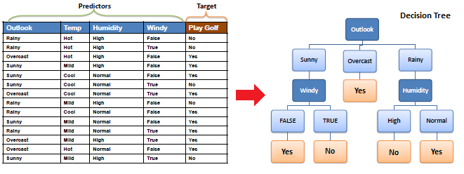
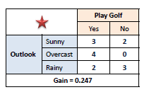
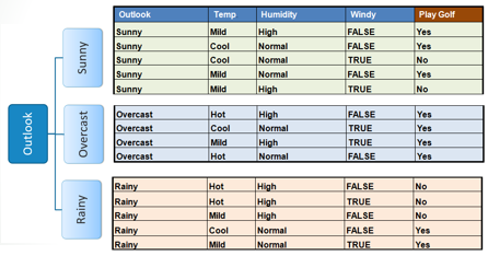
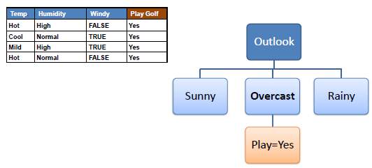
Decision tree builds classification or regression models in the form of a tree structure. It breaks down a dataset into smaller and smaller subsets while at the same time an associated decision tree is incrementally developed. The final result is a tree with decision nodes and leaf nodes. A decision node (e.g., Outlook) has two or more branches (e.g., Sunny, Overcast and Rainy). Leaf node (e.g., Play) represents a classification or decision. The topmost decision node in a tree which corresponds to the best predictor called root node. Decision trees can handle both categorical and numerical data.
Algorithm
The core algorithm for building decision trees called ID3 by J. R. Quinlan which employs a top-down, greedy search through the space of possible branches with no backtracking. ID3 uses Entropy and Information Gain to construct a decision tree. In ZeroR model there is no predictor, in OneR model we try to find the single best predictor, naive Bayesian includes all predictors using Bayes' rule and the independence assumptions between predictors but decision tree includes all predictors with the dependence assumptions between predictors.
Entropy
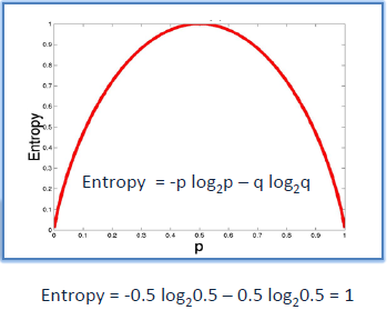
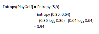
A decision tree is built top-down from a root node and involves partitioning the data into subsets that contain instances with similar values (homogenous). ID3 algorithm uses entropy to calculate the homogeneity of a sample. If the sample is completely homogeneous the entropy is zero and if the sample is an equally divided it has entropy of one.
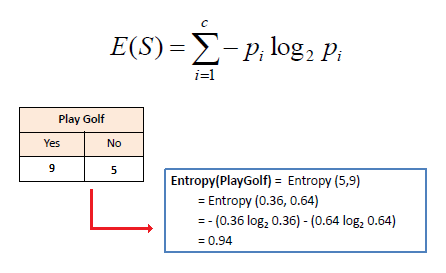
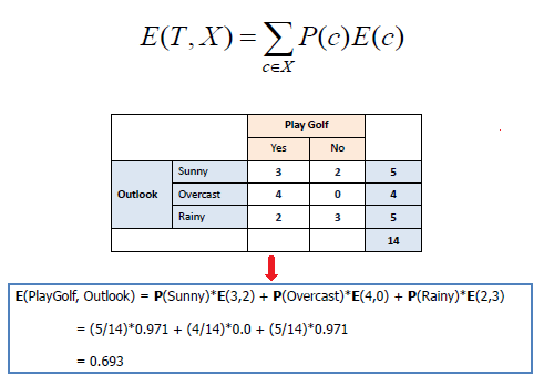
To build a decision tree, we need to calculate two types of entropy using frequency tables as follows:
a) Entropy using the frequency table of one attribute:
b) Entropy using the frequency table of two attributes:
Information Gain
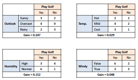
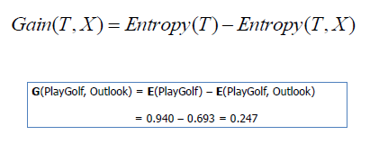
The information gain is based on the decrease in entropy after a dataset is split on an attribute. Constructing a decision tree is all about finding attribute that returns the highest information gain (i.e., the most homogeneous branches).
Step 1: Calculate entropy of the target.
Step 2: The dataset is then split on the different attributes. The entropy for each branch is calculated. Then it is added proportionally, to get total entropy for the split. The resulting entropy is subtracted from the entropy before the split. The result is the Information Gain, or decrease in entropy.
Step 3: Choose attribute with the largest information gain as the decision node, divide the dataset by its branches and repeat the same process on every branch.
Step 4a: A branch with entropy of 0 is a leaf node.
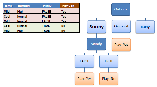
Step 4b: A branch with entropy more than 0 needs further splitting.
Step 5: The ID3 algorithm is run recursively on the non-leaf branches, until all data is classified.
Decision Tree to Decision Rules
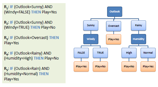
A decision tree can easily be transformed to a set of rules by mapping from the root node to the leaf nodes one by one.
Decision Trees - Issues
Working with continuous attributes (binning) Avoiding overfitting Super Attributes (attributes with many unique values) Working with missing values

Hypothesis space search in Decision Tree Learning Algorithm

In most supervised machine learning algorithm, our main goal is to find out a possible hypothesis from the hypothesis space that could possibly map out the inputs to the proper outputs.
The following figure shows the common method to find out the possible hypothesis from the Hypothesis space:

Hypothesis Space (H):
Hypothesis space is the set of all the possible legal hypothesis. This is the set from which the machine learning algorithm would determine the best possible (only one) which would best describe the target function or the outputs.

Hypothesis (h):
A hypothesis is a function that best describes the target in supervised machine learning. The hypothesis that an algorithm would come up depends upon the data and also depends upon the restrictions and bias that we have imposed on the data. To better understand the Hypothesis Space and Hypothesis consider the following coordinate that shows the distribution of some data:

Say suppose we have test data for which we have to determine the outputs or results. The test data is as shown below:

We can predict the outcomes by dividing the coordinate as shown below:

So the test data would yield the following result:

But note here that we could have divided the coordinate plane as:

The way in which the coordinate would be divided depends on the data, algorithm and constraints.

·  All these legal possible ways in which we can divide the coordinate plane to predict the outcome of the test data composes of the Hypothesis Space.

·  Each individual possible way is known as the hypothesis.

Hence, in this example the hypothesis space would be like:

Decision Trees, Inductive Bias and Hyperparameters

Decision Trees

Decision trees are a type of supervised learning algorithm which are used for mainly classification and regression.

They have a tree like structure in which the internal nodes are "tests" for attributes and the branches are the results of the "tests". The leaf nodes will be the class labels i.e., the output of the learner. Given below is the basic structure of a decision tree.

Given below is an example of a decision tree used to decide wether to walk or take the bus. "Walk" and "Bus" are the class labels in this example. The parameters of the model are weather, time and hunger.

As you can see in the above example, we can clearly examine the decision making process involved. This is a major advantage of decision trees- they are transparent models.

Inductive Bias

Before learning a model given a data and a learning algorithm, there are a few assumptions a learner makes about the algorithm. These assumptions are called the inductive bias. It is like the property of the algorithm.

For eg. in the case of decision trees, the depth of the tress is the inductive bias. If the depth of the tree is too low, then there is too much generalisation in the model. Similarly, if the depth of the tree is too much, there is too less generalisation and while testing the model on a new example, we might reach a particular example used to train the model. This may give us incorrect results.

Hyperparameters

In machine learning the hyperparameters are used to control the learning process as compared to parameters which are obtained after training the model on the data. The hyperparameters are independent of the data.

Hyperparameters are set manually before the training of the model. Generally the hyperparameter is chosen using the inductive bias. After we set out hyperparameter, we train on the data and get a trained model. We used the trained model on separate data to "validate" it. Using this, we tune our hyperparameters as per our requirement. A basic flowchart is given below

Issues in Decision Tree Learning:

 Disadvantages of the Decision Tree:

1.  The decision tree contains lots of layers, which makes it complex.
2.  It may have an overfitting issue, which can be resolved using the Random Forest algorithm.
3.  For more class labels, the computational complexity of the decision tree may increase.

What are appropriate problems for Decision tree learning?

Although a variety of decision tree learning methods have been developed with somewhat differing capabilities and requirements, decision tree learning is generally best suited to problems with the following characteristics:

1. Instances are represented by attribute-value pairs:

In the world of decision tree learning, we commonly use attribute-value pairs to represent instances. An instance is defined by a predetermined group of attributes, such as temperature, and its corresponding value, such as hot. Ideally, we want each attribute to have a finite set of distinct values, like hot, mild, or cold. This makes it easy to construct decision trees. However, more advanced versions of the algorithm can accommodate attributes with continuous numerical values, such as representing temperature with a numerical scale.

2. The target function has discrete output values:

The marked objective has distinct outcomes. The decision tree method is ordinarily employed for categorizing Boolean examples, such as yes or no. Decision tree approaches can be readily expanded for acquiring functions with beyond dual conceivable outcome values. A more substantial expansion lets us gain knowledge about aimed objectives with numeric outputs, although the practice of decision trees in this framework is comparatively rare.

3. Disjunctive descriptions may be required:

Decision trees naturally represent disjunctive expressions.

4.The training data may contain errors:

“Techniques of decision tree learning demonstrate high resilience towards discrepancies, including inconsistencies in categorization of sample cases and discrepancies in the feature details that characterize these cases.”

5. The training data may contain missing attribute values:

In certain cases, the input information designed for training might have absent characteristics. Employing decision tree approaches can still be possible despite experiencing unknown features in some training samples. For instance, when considering the level of humidity throughout the day, this information may only be accessible for a specific set of training specimens.

Practical issues in learning decision trees include:

•  Determining how deeply to grow the decision tree,
•  Handling continuous attributes,
•  Choosing an appropriate attribute selection measure,
•  Handling training data with missing attribute values,
•  Handling attributes with differing costs, and
•  Improving computational efficiency.
•  

To build the Decision Tree, CART (Classification and Regression Tree) algorithm is used. It works by selecting the best split at each node based on metrics like Gini impurity or information Gain. In order to create a decision tree. Here are the basic steps of the CART algorithm:

1. The root node of the tree is supposed to be the complete training dataset.
2. Determine the impurity of the data based on each feature present in the dataset. Impurity can be measured using metrics like the Gini index or entropy for classification and Mean squared error, Mean Absolute Error, friedman_mse, or Half Poisson deviance for regression.
3. Then selects the feature that results in the highest information gain or impurity reduction when splitting the data.
4. For each possible value of the selected feature, split the dataset into two subsets (left and right), one where the feature takes on that value, and another where it does not. The split should be designed to create subsets that are as pure as possible with respect to the target variable.
5. Based on the target variable, determine the impurity of each resulting subset.
6. For each subset, repeat steps 2–5 iteratively until a stopping condition is met. For example, the stopping condition could be a maximum tree depth, a minimum number of samples required to make a split or a minimum impurity threshold.
7. Assign the majority class label for classification tasks or the mean value for regression tasks for each terminal node (leaf node) in the tree.

Bayes Theorem in Machine learning

Machine Learning is one of the most emerging technology of Artificial Intelligence. We are living in the 21th century which is completely driven by new technologies and gadgets in which some are yet to be used and few are on its full potential. Similarly, Machine Learning is also a technology that is still in its developing phase. There are lots of concepts that make machine learning a better technology such as supervised learning, unsupervised learning, reinforcement learning, perceptron models, Neural networks, etc. In this article "Bayes Theorem in Machine Learning", we will discuss another most important concept of Machine Learning theorem i.e., Bayes Theorem. But before starting this topic you should have essential understanding of this theorem such as what exactly is Bayes theorem, why it is used in Machine Learning, examples of Bayes theorem in Machine Learning and much more. So, let's start the brief introduction of Bayes theorem.

Introduction to Bayes Theorem in Machine Learning

Bayes theorem is given by an English statistician, philosopher, and Presbyterian minister named Mr. Thomas Bayes in 17^th century. Bayes provides their thoughts in decision theory which is extensively used in important mathematics concepts as Probability. Bayes theorem is also widely used in Machine Learning where we need to predict classes precisely and accurately. An important concept of Bayes theorem named Bayesian method is used to calculate conditional probability in Machine Learning application that includes classification tasks. Further, a simplified version of Bayes theorem (Naïve Bayes classification) is also used to reduce computation time and average cost of the projects.

Bayes theorem is also known with some other name such as Bayes rule or Bayes Law. Bayes theorem helps to determine the probability of an event with random knowledge. It is used to calculate the probability of occurring one event while other one already occurred. It is a best method to relate the condition probability and marginal probability.

In simple words, we can say that Bayes theorem helps to contribute more accurate results.

Bayes Theorem is used to estimate the precision of values and provides a method for calculating the conditional probability. However, it is hypocritically a simple calculation but it is used to easily calculate the conditional probability of events where intuition often fails. Some of the data scientist assumes that Bayes theorem is most widely used in financial industries but it is not like that. Other than financial, Bayes theorem is also extensively applied in health and medical, research and survey industry, aeronautical sector, etc.

What is Bayes Theorem?

Bayes theorem is one of the most popular machine learning concepts that helps to calculate the probability of occurring one event with uncertain knowledge while other one has already occurred.

Bayes' theorem can be derived using product rule and conditional probability of event X with known event Y:

• According to the product rule we can express as the probability of event X with known event Y as follows;

1.       P(X ? Y)= P(X|Y) P(Y)       {equation 1}  

 

1.       P(X ? Y)= P(Y|X) P(X)       {equation 2}  

Mathematically, Bayes theorem can be expressed by combining both equations on right hand side. We will get:

Here, both events X and Y are independent events which means probability of outcome of both events does not depends one another.

The above equation is called as Bayes Rule or Bayes Theorem.

• P(X|Y) is called as posterior, which we need to calculate. It is defined as updated probability after considering the evidence.
• P(Y|X) is called the likelihood. It is the probability of evidence when hypothesis is true.
• P(X) is called the prior probability, probability of hypothesis before considering the evidence
• P(Y) is called marginal probability. It is defined as the probability of evidence under any consideration.

Hence, Bayes Theorem can be written as:

posterior = likelihood * prior / evidence

Prerequisites for Bayes Theorem

While studying the Bayes theorem, we need to understand few important concepts. These are as follows:

1. Experiment

An experiment is defined as the planned operation carried out under controlled condition such as tossing a coin, drawing a card and rolling a dice, etc.

2. Sample Space

During an experiment what we get as a result is called as possible outcomes and the set of all possible outcome of an event is known as sample space. For example, if we are rolling a dice, sample space will be:

AD

S1 = {1, 2, 3, 4, 5, 6}

Similarly, if our experiment is related to toss a coin and recording its outcomes, then sample space will be:

S2 = {Head, Tail}

3. Event

Event is defined as subset of sample space in an experiment. Further, it is also called as set of outcomes.

AD

Assume in our experiment of rolling a dice, there are two event A and B such that;

A = Event when an even number is obtained = {2, 4, 6}

B = Event when a number is greater than 4 = {5, 6}

• Probability of the event A ''P(A)''= Number of favourable outcomes / Total number of possible outcomes
  P(E) = 3/6 =1/2 =0.5
• Similarly, Probability of the event B ''P(B)''= Number of favourable outcomes / Total number of possible outcomes
  =2/6
  =1/3
  =0.333
• Union of event A and B:
  A∪B = {2, 4, 5, 6}
  
  
  
  
  
• Intersection of event A and B:
  A∩B= {6}
  
  
  
  
  
• Disjoint Event: If the intersection of the event A and B is an empty set or null then such events are known as disjoint event or mutually exclusive events also.
  
  
  
  
  

4. Random Variable:

It is a real value function which helps mapping between sample space and a real line of an experiment. A random variable is taken on some random values and each value having some probability. However, it is neither random nor a variable but it behaves as a function which can either be discrete, continuous or combination of both.

5. Exhaustive Event:

As per the name suggests, a set of events where at least one event occurs at a time, called exhaustive event of an experiment.

Thus, two events A and B are said to be exhaustive if either A or B definitely occur at a time and both are mutually exclusive for e.g., while tossing a coin, either it will be a Head or may be a Tail.

6. Independent Event:

Two events are said to be independent when occurrence of one event does not affect the occurrence of another event. In simple words we can say that the probability of outcome of both events does not depends one another.

Mathematically, two events A and B are said to be independent if:

P(A ∩ B) = P(AB) = P(A)*P(B)

7. Conditional Probability:

Conditional probability is defined as the probability of an event A, given that another event B has already occurred (i.e. A conditional B). This is represented by P(A|B) and we can define it as:

P(A|B) = P(A ∩ B) / P(B)

8. Marginal Probability:

Marginal probability is defined as the probability of an event A occurring independent of any other event B. Further, it is considered as the probability of evidence under any consideration.

P(A) = P(A|B)*P(B) + P(A|~B)*P(~B)

Here ~B represents the event that B does not occur.

AD

How to apply Bayes Theorem or Bayes rule in Machine Learning?

Bayes theorem helps us to calculate the single term P(B|A) in terms of P(A|B), P(B), and P(A). This rule is very helpful in such scenarios where we have a good probability of P(A|B), P(B), and P(A) and need to determine the fourth term.

Naïve Bayes classifier is one of the simplest applications of Bayes theorem which is used in classification algorithms to isolate data as per accuracy, speed and classes.

Let's understand the use of Bayes theorem in machine learning with below example.

Suppose, we have a vector A with I attributes. It means

A = A1, A2, A3, A4……………Ai

Further, we have n classes represented as C1, C2, C3, C4…………Cn.

These are two conditions given to us, and our classifier that works on Machine Language has to predict A and the first thing that our classifier has to choose will be the best possible class. So, with the help of Bayes theorem, we can write it as:

P(Ci/A)= [ P(A/Ci) * P(Ci)] / P(A)

Here;

P(A) is the condition-independent entity.

P(A) will remain constant throughout the class means it does not change its value with respect to change in class. To maximize the P(Ci/A), we have to maximize the value of term P(A/Ci) * P(Ci).

With n number classes on the probability list let's assume that the possibility of any class being the right answer is equally likely. Considering this factor, we can say that:

P(C1)=P(C2)-P(C3)=P(C4)=…..=P(Cn).

This process helps us to reduce the computation cost as well as time. This is how Bayes theorem plays a significant role in Machine Learning and Naïve Bayes theorem has simplified the conditional probability tasks without affecting the precision. Hence, we can conclude that:

P(Ai/C)= P(A1/C)* P(A2/C)* P(A3/C)*……*P(An/C)

Hence, by using Bayes theorem in Machine Learning we can easily describe the possibilities of smaller events.

What is Naïve Bayes Classifier in Machine Learning

Naïve Bayes theorem is also a supervised algorithm, which is based on Bayes theorem and used to solve classification problems. It is one of the most simple and effective classification algorithms in Machine Learning which enables us to build various ML models for quick predictions. It is a probabilistic classifier that means it predicts on the basis of probability of an object. Some popular Naïve Bayes algorithms are spam filtration, Sentimental analysis, and classifying articles.

Advantages of Naïve Bayes Classifier in Machine Learning:

• It is one of the simplest and effective methods for calculating the conditional probability and text classification problems.
• A Naïve-Bayes classifier algorithm is better than all other models where assumption of independent predictors holds true.
• It is easy to implement than other models.
• It requires small amount of training data to estimate the test data which minimize the training time period.
• It can be used for Binary as well as Multi-class Classifications.

Disadvantages of Naïve Bayes Classifier in Machine Learning:

The main disadvantage of using Naïve Bayes classifier algorithms is, it limits the assumption of independent predictors because it implicitly assumes that all attributes are independent or unrelated but in real life it is not feasible to get mutually independent attributes.

Conclusion

Though, we are living in technology world where everything is based on various new technologies that are in developing phase but still these are incomplete in absence of already available classical theorems and algorithms. Bayes theorem is also most popular example that is used in Machine Learning. Bayes theorem has so many applications in Machine Learning. In classification related problems, it is one of the most preferred methods than all other algorithm. Hence, we can say that Machine Learning is highly dependent on Bayes theorem. In this article, we have discussed about Bayes theorem, how can we apply Bayes theorem in Machine Learning, Naïve Bayes Classifier, etc.

 

Maximum Likelihood Estimation (MLE) and Least Squares Error (LSE)

Maximum Likelihood Estimation (MLE) and Least Squares Error (LSE) are both methods used in statistical estimation, but they are commonly associated with different types of problems.

1. Maximum Likelihood Estimation (MLE):

   • Objective: MLE is a method used to estimate the parameters of a statistical model by maximizing the likelihood function. The likelihood function represents the probability of observing the given data under the assumed model.
   • Methodology: The idea is to find the values of the model parameters that make the observed data most probable. This is often equivalent to finding the parameters that maximize the product of the probabilities of the observed data points.
   • Application: MLE is widely used in various statistical models, such as linear regression, logistic regression, and many other parametric models.

2. Least Squares Error (LSE):

   • Objective: LSE is a method used for estimating the parameters of a model by minimizing the sum of the squared differences between the observed and predicted values.
   • Methodology: In the context of linear regression, for example, the goal is to find the line that minimizes the sum of the squared vertical distances (residuals) between the observed data points and the points on the line.
   • Application: LSE is commonly used in linear regression, where the relationship between the dependent and independent variables is assumed to be linear. The parameters are chosen to minimize the sum of squared residuals.

In summary, MLE is more general and can be applied to a broader range of statistical models, while LSE is specifically associated with minimizing the sum of squared errors and is commonly used in linear regression. The choice between MLE and LSE depends on the nature of the problem and the assumptions about the underlying model.

Maximum Likelihood Estimation (MLE) and Least Squares Error (LSE) are two common statistical methods used to estimate model parameters from data. Both methods aim to find the values of the parameters that make the observed data as likely as possible. However, they differ in their underlying assumptions and their optimization goals.

Maximum Likelihood Estimation (MLE)

MLE is a statistical method that estimates model parameters by maximizing the likelihood of the observed data. The likelihood function measures the probability of observing the data given the model parameters. The MLE approach finds the values of the parameters that maximize the likelihood function, indicating that these parameters are the most likely to have produced the observed data.

Least Squares Error (LSE)

LSE is a statistical method that estimates model parameters by minimizing the sum of the squared errors between the observed data and the predicted values from the model. The squared error is a measure of the discrepancy between the observed and predicted values. The LSE approach finds the values of the parameters that minimize the total squared error, indicating that these parameters produce the best fit between the model and the data.

Differences between MLE and LSE

• Distributional assumptions: MLE typically assumes that the data follows a specific probability distribution, such as the normal distribution. LSE does not require any specific distributional assumptions, but it performs better when the errors are normally distributed.

• Optimization goals: MLE maximizes the likelihood of the observed data, while LSE minimizes the sum of squared errors.

• Estimator properties: MLE estimators are asymptotically unbiased and consistent, meaning that they converge to the true parameter values as the sample size increases. LSE estimators are unbiased and consistent under the assumption of normally distributed errors.

Applications of MLE and LSE

MLE and LSE are widely used in various statistical applications, including:

• Linear regression: Both MLE and LSE can be used to estimate the coefficients in a linear regression model.

• Logistic regression: MLE is commonly used to estimate the coefficients in a logistic regression model.

• Time series analysis: MLE is frequently used to estimate the parameters of time series models.

Choosing between MLE and LSE

The choice between MLE and LSE depends on the specific context and the assumptions of the model. If the data is assumed to follow a specific distribution and the goal is to maximize the likelihood of the data, then MLE is the appropriate method. However, if the distributional assumptions are uncertain or the goal is to minimize the sum of squared errors, then LSE is a more suitable choice.

The Minimum Description Length (MDL) principle is a statistical and information-theoretic approach to model selection and inductive inference. It asserts that the best explanation for a given set of data is the one that achieves the shortest possible description length. In other words, the MDL principle states that the simplest model that can accurately represent the data is the best model.

The MDL principle is based on the idea that the best explanation for any phenomenon is the one that can be encoded using the fewest bits. This principle has a strong foundation in information theory, which states that the amount of information contained in a message is inversely proportional to its compression ratio.

The MDL principle has been applied to a wide variety of problems in machine learning, statistics, and artificial intelligence. It has been shown to be effective in tasks such as model selection, parameter estimation, and data compression.

The MDL principle is a powerful tool for understanding the relationship between data and complexity. It provides a principled way to select models that are both accurate and parsimonious.

Key concepts of MDL

• Description length: The description length of a model is the sum of the length of the model itself and the length of the encoded data.

• Model complexity: The complexity of a model is related to the number of parameters it has. A more complex model has more parameters and can therefore capture more complex relationships in the data.

• Overfitting: Overfitting occurs when a model is too complex and fits the training data too well, leading to poor performance on new data.

Benefits of MDL

• MDL can prevent overfitting. By selecting the simplest model that can accurately represent the data, MDL can help to avoid overfitting and improve the generalization performance of models.

• MDL can be used to compare models of different complexity. MDL provides a consistent framework for comparing models of different complexity, making it easier to select the best model for a given task.

• MDL is a principled approach to model selection. MDL is based on a strong theoretical foundation in information theory, making it a principled approach to model selection.

Applications of MDL

• Model selection: MDL can be used to select the best model from a set of candidate models.

• Parameter estimation: MDL can be used to estimate the parameters of a model.

• Data compression: MDL can be used to compress data by selecting the most efficient representation of the data.

The Minimum Description Length (MDL) principle is a concept used in information theory and statistics for model selection and hypothesis testing. It was introduced by Jorma Rissanen in the 1970s. The MDL principle is based on the idea that the best model is the one that allows for the most concise representation of the data.

Here's a simplified explanation of the MDL principle:

1. Description Length:

   • The "description length" refers to the length of the code or representation needed to convey both the model and the data.
   • A shorter description length implies a more efficient and concise representation.

2. Two Parts of Description Length:

   • Model Length: The length of the code required to describe the chosen model.
   • Data Length: The length of the code required to describe the data given the chosen model.

3. Principle:

   • The MDL principle suggests that the best model is the one that minimizes the total description length, which is the sum of the model length and the data length.
   • The principle seeks a balance between the complexity of the model and its ability to accurately describe the data.

4. Model Selection:

   • In the context of model selection, the MDL principle can be used to compare different models. The model with the shortest total description length is considered the best, as it effectively captures the data without unnecessary complexity.

5. Hypothesis Testing:

   • In the context of hypothesis testing, the MDL principle can be used to choose between competing hypotheses. The hypothesis that results in the shortest total description length is favored.

6. Application:

   • MDL has been applied in various fields, including machine learning, statistics, and data compression. It provides a theoretically grounded approach to balancing model complexity and data fit.

In summary, the Minimum Description Length principle is a concept that seeks to find a model that provides a concise and efficient representation of both the model and the observed data. It is a general principle applicable to various areas where model selection and hypothesis testing are crucial.

Naive Bayes Classifier:

Gibbs Algorithm

• Bayes optimal classifier provides best result, but can be expensive if many hypotheses.
• Gibbs algorithm:
  1. Choose one hypothesis at random, according to $P(h\,|\,D)$
  2. Use this to classify new instance
• Surprising fact: Assume target concepts are drawn at random from $H$ according to priors on $H$. Then: \[ E[error_{Gibbs}] \leq 2 E[error_{Bayes Optimal}] \] So, if the learner correctly assumes a uniform prior distribution over $H$, then
• Pick any hypothesis from VS, with uniform probability
• Its expected error is no worse than twice Bayes optimal

Here's a simple explanation of the Gibbs sampling algorithm:

1. Initialize: Start with an initial guess of the parameters.

2. Iterate:

   • For each variable in the distribution:
     • Sample from the conditional distribution of that variable given the current values of the other variables.

3. Repeat: Repeat the iteration process for a sufficient number of steps until convergence.

Gibbs sampling is often employed in Bayesian models, where it helps in sampling from the posterior distribution of parameters given observed data.

Please note that while Gibbs sampling is widely used, the term "Gibbs algorithm" might be used in various contexts, so it's always a good idea to check the specific details or context in which it's being mentioned.

Advantages of Gibbs Sampling

• Adaptability: Gibbs sampling can be applied to a wide range of probability distributions, including complex multivariate distributions.

• Efficiency: Gibbs sampling is often more efficient than other MCMC methods, such as the Metropolis-Hastings algorithm.

• Versatility: Gibbs sampling can be used for a variety of statistical tasks, including parameter estimation, Bayesian inference, and simulation.

Applications of Gibbs Sampling

• Bayesian inference: Gibbs sampling is a powerful tool for performing Bayesian inference, which involves updating beliefs about parameters based on observed data.

• Latent variable models: Gibbs sampling is widely used for fitting latent variable models, which include latent Dirichlet allocation (LDA) and topic models.

• Machine learning: Gibbs sampling can be used for unsupervised learning tasks, such as clustering and dimensionality reduction.

Example of Gibbs Sampling for Bayesian Inference

Consider a simple Bayesian model where we want to estimate the mean and variance of a set of observed data points. We can assume a normal distribution for the data and use a hierarchical prior for the mean and variance. The Gibbs sampling algorithm would then iterate by sampling the mean and variance from their respective conditional distributions, given the current values of the data points and the other parameters.

EM Algorithm in Machine Learning

The EM algorithm is considered a latent variable model to find the local maximum likelihood parameters of a statistical model, proposed by Arthur Dempster, Nan Laird, and Donald Rubin in 1977. The EM (Expectation-Maximization) algorithm is one of the most commonly used terms in machine learning to obtain maximum likelihood estimates of variables that are sometimes observable and sometimes not. However, it is also applicable to unobserved data or sometimes called latent. It has various real-world applications in statistics, including obtaining the mode of the posterior marginal distribution of parameters in machine learning and data mining applications.

In most real-life applications of machine learning, it is found that several relevant learning features are available, but very few of them are observable, and the rest are unobservable. If the variables are observable, then it can predict the value using instances. On the other hand, the variables which are latent or directly not observable, for such variables Expectation-Maximization (EM) algorithm plays a vital role to predict the value with the condition that the general form of probability distribution governing those latent variables is known to us. In this topic, we will discuss a basic introduction to the EM algorithm, a flow chart of the EM algorithm, its applications, advantages, and disadvantages of EM algorithm, etc.

What is an EM algorithm?

The Expectation-Maximization (EM) algorithm is defined as the combination of various unsupervised machine learning algorithms, which is used to determine the local maximum likelihood estimates (MLE) or maximum a posteriori estimates (MAP) for unobservable variables in statistical models. Further, it is a technique to find maximum likelihood estimation when the latent variables are present. It is also referred to as the latent variable model.

A latent variable model consists of both observable and unobservable variables where observable can be predicted while unobserved are inferred from the observed variable. These unobservable variables are known as latent variables.

Key Points:

• It is known as the latent variable model to determine MLE and MAP parameters for latent variables.
• It is used to predict values of parameters in instances where data is missing or unobservable for learning, and this is done until convergence of the values occurs.

EM Algorithm

The EM algorithm is the combination of various unsupervised ML algorithms, such as the k-means clustering algorithm. Being an iterative approach, it consists of two modes. In the first mode, we estimate the missing or latent variables. Hence it is referred to as the Expectation/estimation step (E-step). Further, the other mode is used to optimize the parameters of the models so that it can explain the data more clearly. The second mode is known as the maximization-step or M-step.

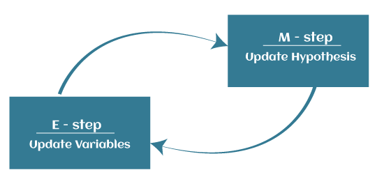
• Expectation step (E - step): It involves the estimation (guess) of all missing values in the dataset so that after completing this step, there should not be any missing value.
• Maximization step (M - step): This step involves the use of estimated data in the E-step and updating the parameters.
• Repeat E-step and M-step until the convergence of the values occurs.

The primary goal of the EM algorithm is to use the available observed data of the dataset to estimate the missing data of the latent variables and then use that data to update the values of the parameters in the M-step.

What is Convergence in the EM algorithm?

Convergence is defined as the specific situation in probability based on intuition, e.g., if there are two random variables that have very less difference in their probability, then they are known as converged. In other words, whenever the values of given variables are matched with each other, it is called convergence.

Steps in EM Algorithm

The EM algorithm is completed mainly in 4 steps, which include Initialization Step, Expectation Step, Maximization Step, and convergence Step. These steps are explained as follows:

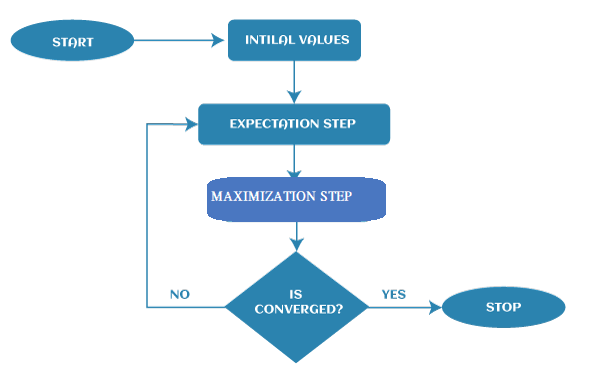
• 1^st Step: The very first step is to initialize the parameter values. Further, the system is provided with incomplete observed data with the assumption that data is obtained from a specific model.

• 2^nd Step: This step is known as Expectation or E-Step, which is used to estimate or guess the values of the missing or incomplete data using the observed data. Further, E-step primarily updates the variables.
• 3^rd Step: This step is known as Maximization or M-step, where we use complete data obtained from the 2^nd step to update the parameter values. Further, M-step primarily updates the hypothesis.
• 4^th step: The last step is to check if the values of latent variables are converging or not. If it gets "yes", then stop the process; else, repeat the process from step 2 until the convergence occurs.

Gaussian Mixture Model (GMM)

The Gaussian Mixture Model or GMM is defined as a mixture model that has a combination of the unspecified probability distribution function. Further, GMM also requires estimated statistics values such as mean and standard deviation or parameters. It is used to estimate the parameters of the probability distributions to best fit the density of a given training dataset. Although there are plenty of techniques available to estimate the parameter of the Gaussian Mixture Model (GMM), the Maximum Likelihood Estimation is one of the most popular techniques among them.

Let's understand a case where we have a dataset with multiple data points generated by two different processes. However, both processes contain a similar Gaussian probability distribution and combined data. Hence it is very difficult to discriminate which distribution a given point may belong to.

The processes used to generate the data point represent a latent variable or unobservable data. In such cases, the Estimation-Maximization algorithm is one of the best techniques which helps us to estimate the parameters of the gaussian distributions. In the EM algorithm, E-step estimates the expected value for each latent variable, whereas M-step helps in optimizing them significantly using the Maximum Likelihood Estimation (MLE). Further, this process is repeated until a good set of latent values, and a maximum likelihood is achieved that fits the data.

Applications of EM algorithm

The primary aim of the EM algorithm is to estimate the missing data in the latent variables through observed data in datasets. The EM algorithm or latent variable model has a broad range of real-life applications in machine learning. These are as follows:

• The EM algorithm is applicable in data clustering in machine learning.
• It is often used in computer vision and NLP (Natural language processing).
• It is used to estimate the value of the parameter in mixed models such as the Gaussian Mixture Modeland quantitative genetics.
• It is also used in psychometrics for estimating item parameters and latent abilities of item response theory models.
• It is also applicable in the medical and healthcare industry, such as in image reconstruction and structural engineering.
• It is used to determine the Gaussian density of a function.

Advantages of EM algorithm

• It is very easy to implement the first two basic steps of the EM algorithm in various machine learning problems, which are E-step and M- step.
• It is mostly guaranteed that likelihood will enhance after each iteration.
• It often generates a solution for the M-step in the closed form.

Disadvantages of EM algorithm

• The convergence of the EM algorithm is very slow.
• It can make convergence for the local optima only.
• It takes both forward and backward probability into consideration. It is opposite to that of numerical optimization, which takes only forward probabilities.

Conclusion

In real-world applications of machine learning, the expectation-maximization (EM) algorithm plays a significant role in determining the local maximum likelihood estimates (MLE) or maximum a posteriori estimates (MAP) for unobservable variables in statistical models. It is often used for the latent variables, i.e., to estimate the latent variables through observed data in datasets. It is generally completed in two important steps, i.e., the expectation step (E-step) and the Maximization step (M-Step), where E-step is used to estimate the missing data in datasets, and M-step is used to update the parameters after the complete data is generated in E-step. Further, the importance of the EM algorithm can be seen in various applications such as data clustering, natural language processing (NLP), computer vision, image reconstruction, structural engineering, etc.

Artificial Neural Network Tutorial

Artificial Neural Network Tutorial provides basic and advanced concepts of ANNs. Our Artificial Neural Network tutorial is developed for beginners as well as professions.

The term "Artificial neural network" refers to a biologically inspired sub-field of artificial intelligence modeled after the brain. An Artificial neural network is usually a computational network based on biological neural networks that construct the structure of the human brain. Similar to a human brain has neurons interconnected to each other, artificial neural networks also have neurons that are linked to each other in various layers of the networks. These neurons are known as nodes.

Artificial neural network tutorial covers all the aspects related to the artificial neural network. In this tutorial, we will discuss ANNs, Adaptive resonance theory, Kohonen self-organizing map, Building blocks, unsupervised learning, Genetic algorithm, etc.

What is Artificial Neural Network?

The term "Artificial Neural Network" is derived from Biological neural networks that develop the structure of a human brain. Similar to the human brain that has neurons interconnected to one another, artificial neural networks also have neurons that are interconnected to one another in various layers of the networks. These neurons are known as nodes.

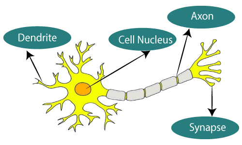
The given figure illustrates the typical diagram of Biological Neural Network.

The typical Artificial Neural Network looks something like the given figure.

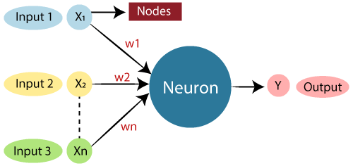
Dendrites from Biological Neural Network represent inputs in Artificial Neural Networks, cell nucleus represents Nodes, synapse represents Weights, and Axon represents Output.

Relationship between Biological neural network and artificial neural network:

Biological Neural Network	Artificial Neural Network
Dendrites	Inputs
Cell nucleus	Nodes
Synapse	Weights
Axon	Output

An Artificial Neural Network in the field of Artificial intelligence where it attempts to mimic the network of neurons makes up a human brain so that computers will have an option to understand things and make decisions in a human-like manner. The artificial neural network is designed by programming computers to behave simply like interconnected brain cells.

There are around 1000 billion neurons in the human brain. Each neuron has an association point somewhere in the range of 1,000 and 100,000. In the human brain, data is stored in such a manner as to be distributed, and we can extract more than one piece of this data when necessary from our memory parallelly. We can say that the human brain is made up of incredibly amazing parallel processors.

We can understand the artificial neural network with an example, consider an example of a digital logic gate that takes an input and gives an output. "OR" gate, which takes two inputs. If one or both the inputs are "On," then we get "On" in output. If both the inputs are "Off," then we get "Off" in output. Here the output depends upon input. Our brain does not perform the same task. The outputs to inputs relationship keep changing because of the neurons in our brain, which are "learning."

The architecture of an artificial neural network:

To understand the concept of the architecture of an artificial neural network, we have to understand what a neural network consists of. In order to define a neural network that consists of a large number of artificial neurons, which are termed units arranged in a sequence of layers. Lets us look at various types of layers available in an artificial neural network.

Artificial Neural Network primarily consists of three layers:

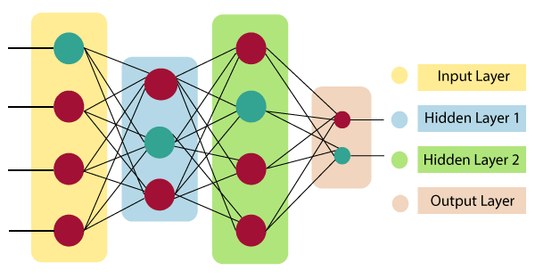
Input Layer:

As the name suggests, it accepts inputs in several different formats provided by the programmer.

Hidden Layer:

The hidden layer presents in-between input and output layers. It performs all the calculations to find hidden features and patterns.

Output Layer:

The input goes through a series of transformations using the hidden layer, which finally results in output that is conveyed using this layer.

The artificial neural network takes input and computes the weighted sum of the inputs and includes a bias. This computation is represented in the form of a transfer function.

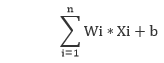
It determines weighted total is passed as an input to an activation function to produce the output. Activation functions choose whether a node should fire or not. Only those who are fired make it to the output layer. There are distinctive activation functions available that can be applied upon the sort of task we are performing.

Advantages of Artificial Neural Network (ANN)

Parallel processing capability:

Artificial neural networks have a numerical value that can perform more than one task simultaneously.

Storing data on the entire network:

Data that is used in traditional programming is stored on the whole network, not on a database. The disappearance of a couple of pieces of data in one place doesn't prevent the network from working.

Capability to work with incomplete knowledge:

After ANN training, the information may produce output even with inadequate data. The loss of performance here relies upon the significance of missing data.

Having a memory distribution:

For ANN is to be able to adapt, it is important to determine the examples and to encourage the network according to the desired output by demonstrating these examples to the network. The succession of the network is directly proportional to the chosen instances, and if the event can't appear to the network in all its aspects, it can produce false output.

Having fault tolerance:

Extortion of one or more cells of ANN does not prohibit it from generating output, and this feature makes the network fault-tolerance.

Disadvantages of Artificial Neural Network:

Assurance of proper network structure:

There is no particular guideline for determining the structure of artificial neural networks. The appropriate network structure is accomplished through experience, trial, and error.

Unrecognized behavior of the network:

It is the most significant issue of ANN. When ANN produces a testing solution, it does not provide insight concerning why and how. It decreases trust in the network.

Hardware dependence:

Artificial neural networks need processors with parallel processing power, as per their structure. Therefore, the realization of the equipment is dependent.

Difficulty of showing the issue to the network:

ANNs can work with numerical data. Problems must be converted into numerical values before being introduced to ANN. The presentation mechanism to be resolved here will directly impact the performance of the network. It relies on the user's abilities.

The duration of the network is unknown:

The network is reduced to a specific value of the error, and this value does not give us optimum results.

Science artificial neural networks that have steeped into the world in the mid-20^th century are exponentially developing. In the present time, we have investigated the pros of artificial neural networks and the issues encountered in the course of their utilization. It should not be overlooked that the cons of ANN networks, which are a flourishing science branch, are eliminated individually, and their pros are increasing day by day. It means that artificial neural networks will turn into an irreplaceable part of our lives progressively important.

How do artificial neural networks work?

Artificial Neural Network can be best represented as a weighted directed graph, where the artificial neurons form the nodes. The association between the neurons outputs and neuron inputs can be viewed as the directed edges with weights. The Artificial Neural Network receives the input signal from the external source in the form of a pattern and image in the form of a vector. These inputs are then mathematically assigned by the notations x(n) for every n number of inputs.

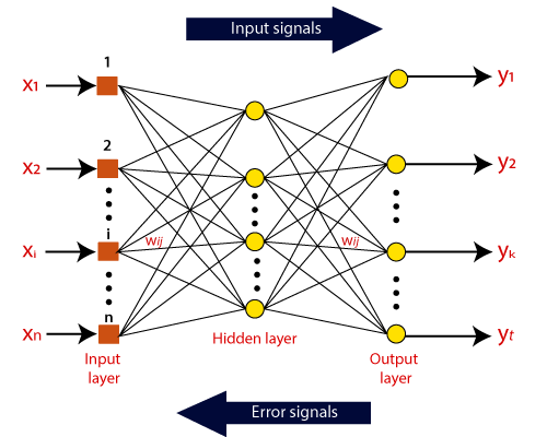
Afterward, each of the input is multiplied by its corresponding weights ( these weights are the details utilized by the artificial neural networks to solve a specific problem ). In general terms, these weights normally represent the strength of the interconnection between neurons inside the artificial neural network. All the weighted inputs are summarized inside the computing unit.

If the weighted sum is equal to zero, then bias is added to make the output non-zero or something else to scale up to the system's response. Bias has the same input, and weight equals to 1. Here the total of weighted inputs can be in the range of 0 to positive infinity. Here, to keep the response in the limits of the desired value, a certain maximum value is benchmarked, and the total of weighted inputs is passed through the activation function.

The activation function refers to the set of transfer functions used to achieve the desired output. There is a different kind of the activation function, but primarily either linear or non-linear sets of functions. Some of the commonly used sets of activation functions are the Binary, linear, and Tan hyperbolic sigmoidal activation functions. Let us take a look at each of them in details:

Binary:

In binary activation function, the output is either a one or a 0. Here, to accomplish this, there is a threshold value set up. If the net weighted input of neurons is more than 1, then the final output of the activation function is returned as one or else the output is returned as 0.

Sigmoidal Hyperbolic:

The Sigmoidal Hyperbola function is generally seen as an "S" shaped curve. Here the tan hyperbolic function is used to approximate output from the actual net input. The function is defined as:

F(x) = (1/1 + exp(-????x))

Where ???? is considered the Steepness parameter.

Types of Artificial Neural Network:

There are various types of Artificial Neural Networks (ANN) depending upon the human brain neuron and network functions, an artificial neural network similarly performs tasks. The majority of the artificial neural networks will have some similarities with a more complex biological partner and are very effective at their expected tasks. For example, segmentation or classification.

Feedback ANN:

In this type of ANN, the output returns into the network to accomplish the best-evolved results internally. As per the University of Massachusetts, Lowell Centre for Atmospheric Research. The feedback networks feed information back into itself and are well suited to solve optimization issues. The Internal system error corrections utilize feedback ANNs.

Feed-Forward ANN:

A feed-forward network is a basic neural network comprising of an input layer, an output layer, and at least one layer of a neuron. Through assessment of its output by reviewing its input, the intensity of the network can be noticed based on group behavior of the associated neurons, and the output is decided. The primary advantage of this network is that it figures out how to evaluate and recognize input patterns.

Prerequisite

No specific expertise is needed as a prerequisite before starting this tutorial.

Audience

Our Artificial Neural Network Tutorial is developed for beginners as well as professionals, to help them understand the basic concept of ANNs.

Problems

We assure you that you will not find any problem in this Artificial Neural Network tutorial. But if there is any problem or mistake, please post the problem in the contact form so that we can further improve it.

Appropriate Problems for ANN

• training data is noisy, complex sensor data
• also problems where symbolic algos are used (decision tree learning (DTL)) - ANN and DTL produce results of comparable accuracy
• instances are attribute-value pairs, attributes may be highly correlated or independent, values can be any real value
• target function may be discrete-valued, real-valued or a vector
• training examples may contain errors
• long training times are acceptable
• requires fast eval. of learned target func.
• humans do NOT need to understand the learned target func.

Artificial Neural Networks (ANNs) are a powerful tool for solving diverse problems, but they are not suited for every task. Here are the key characteristics of problems for which ANNs are particularly well-suited:

1. Non-linear and Complex Relationships:

• ANNs excel at identifying patterns and relationships in data that are non-linear or highly complex, tasks that traditional linear models often struggle with.
• Examples: Image recognition, speech recognition, natural language processing, financial forecasting, medical diagnosis.

2. Learning from Data:

• ANNs can learn directly from data without requiring explicit programming of rules or decision trees. They construct their own internal representations of the data through training.
• Examples: Detecting anomalies in sensor readings, predicting customer behavior, classifying objects in images.

3. Robustness to Noise and Missing Data:

• ANNs have a degree of tolerance for noise and incompleteness in data. They can still extract meaningful patterns even when some information is missing or imperfect.
• Examples: Image denoising, text completion, predicting outcomes in scenarios with uncertain inputs.

4. Generalization:

• Well-trained ANNs can generalize well to new, unseen data, meaning they can make accurate predictions or decisions even on examples they haven't encountered during training.
• Examples: Self-driving cars, machine translation, speech synthesis.

5. Fast Evaluation:

• Once trained, ANNs can make predictions or decisions very quickly. This makes them well-suited for real-time applications that require immediate responses.
• Examples: Fraud detection, spam filtering, real-time recommendations.

However, ANNs may not be optimal for tasks where:

• Interpretability is crucial: It's often difficult to explain why an ANN made a particular decision, which can be a drawback in domains where transparency is essential (e.g., medical diagnosis, legal decision-making).
• Data is limited: ANNs typically require large amounts of training data to perform well. If data is scarce, other machine learning methods might be more suitable.
• Real-time constraints are extremely strict: While ANNs can make fast evaluations, they may have a slight latency compared to simpler models, potentially posing challenges for tasks with extreme real-time demands.

In summary, consider the following factors when deciding if ANNs are appropriate for a given problem:

• Nature of the problem: Is it non-linear, complex, and involve difficult-to-define patterns?
• Data availability: Is there sufficient high-quality data for training?
• Interpretability requirements: Is it necessary to understand the model's reasoning?
• Performance requirements: Are accuracy and speed of decision-making critical?

By carefully evaluating these factors, you can make an informed decision about whether ANNs are the right tool for the job.

డ్రాఫ్ట్ B

Artificial neural networks (ANNs) are a type of machine learning algorithm inspired by the structure and function of the human brain. They excel at tasks that involve pattern recognition, classification, and prediction, and they have been successfully applied to a wide range of problems in various domains.

Here are some of the types of problems that are well-suited for ANNs:

1. Image Recognition: ANNs are particularly adept at recognizing patterns in images, making them well-suited for tasks such as facial recognition, object detection, and image classification.

2. Speech Recognition: ANNs can analyze the acoustic properties of speech and convert them into text, enabling speech-to-text transcription and voice assistant applications.

3. Natural Language Processing (NLP): ANNs can process and understand natural language, enabling tasks such as machine translation, sentiment analysis, and text summarization.

4. Time Series Forecasting: ANNs can learn from historical data to predict future trends, making them useful for forecasting stock prices, weather patterns, and sales figures.

5. Anomaly Detection: ANNs can detect unusual patterns or outliers in data, enabling fraud detection, network intrusion detection, and system maintenance.

6. Recommendation Systems: ANNs can analyze user behavior and preferences to recommend products, movies, or music, tailoring suggestions to individual tastes.

7. Medical Diagnosis: ANNs can assist in medical diagnosis by analyzing medical images, patient records, and laboratory tests, providing risk assessments and treatment recommendations.

8. Robotics and Control Systems: ANNs can control robotic movements, optimize industrial processes, and manage complex systems, adapting to changing conditions and disturbances.

9. Financial Modeling: ANNs can model financial markets, predict market movements, and assess investment risks, providing valuable insights for financial decision-making.

10. Scientific Research: ANNs can analyze large datasets, identify patterns, and make predictions, contributing to various scientific fields such as physics, chemistry, and biology.

These are just a few examples of the many types of problems that ANNs can effectively address. As ANN technology continues to evolve.

Backpropagation

Introduction

The Backpropagation neural network is a multilayered, feedforward neural network and is by far the most extensively used[6]. It is also considered one of the simplest and most general methods used for supervised training of multilayered neural networks[6]. Backpropagation works by approximating the non-linear relationship between the input and the output by adjusting the weight values internally. It can further be generalized for the input that is not included in the training patterns (predictive abilities).

Generally, the Backpropagation network has two stages, training and testing. During the training phase, the network is "shown" sample inputs and the correct classifications. For example, the input might be an encoded picture of a face, and the output could be represented by a code that corresponds to the name of the person.

A further note on encoding information - a neural network, as most learning algorithms, needs to have the inputs and outputs encoded according to an arbitrary user defined scheme. The scheme will define the network architecture so that once a network is trained, the scheme cannot be changed without creating a totally new net. Similarly there are many forms of encoding the network response.

The following figure shows the topology of the Backpropagation neural network that includes and input layer, one hidden layer and an output layer. It should be noted that Backpropagation neural networks can have more than one hidden layer.

Figure 5 Backpropagation Neural Network with one hidden layer[6]

Theory

The operations of the Backpropagation neural networks can be divided into two steps: feedforward and Backpropagation. In the feedforward step, an input pattern is applied to the input layer and its effect propagates, layer by layer, through the network until an output is produced. The network's actual output value is then compared to the expected output, and an error signal is computed for each of the output nodes. Since all the hidden nodes have, to some degree, contributed to the errors evident in the output layer, the output error signals are transmitted backwards from the output layer to each node in the hidden layer that immediately contributed to the output layer. This process is then repeated, layer by layer, until each node in the network has received an error signal that describes its relative contribution to the overall error.

Once the error signal for each node has been determined, the errors are then used by the nodes to update the values for each connection weights until the network converges to a state that allows all the training patterns to be encoded. The Backpropagation algorithm looks for the minimum value of the error function in weight space using a technique called the delta rule or gradient descent[2]. The weights that minimize the error function is then considered to be a solution to the learning problem.

The network behaviour is analogous to a human that is shown a set of data and is asked to classify them into predefined classes. Like a human, it will come up with "theories" about how the samples fit into the classes. These are then tested against the correct outputs to see how accurate the guesses of the network are. Radical changes in the latest theory are indicated by large changes in the weights, and small changes may be seen as minor adjustments to the theory.

There are also issues regarding generalizing a neural network. Issues to consider are problems associated with under-training and over-training data. Under-training can occur when the neural network is not complex enough to detect a pattern in a complicated data set. This is usually the result of networks with so few hidden nodes that it cannot accurately represent the solution, therefore under-fitting the data (Figure 6)[1].
 

Figure 6 Under-fitting data

On the other hand, over-training can result in a network that is too complex, resulting in predictions that are far beyond the range of the training data. Networks with too many hidden nodes will tend to over-fit the solution (Figure 7)[1].
 

Figure 7 Over-fitting data

The aim is to create a neural network with the "right" number of hidden nodes that will lead to a good solution to the problem (Figure 8)[1].
 

Figure 8 Good fit of the data

Algorithm

Using Figure 3, the following describes the learning algorithm and the equations used to train a neural network. For an extensive description on the derivation of the equations used, please refer to reference [10].

Feedforward[10]
When a specified training pattern is fed to the input layer, the weighted sum of the input to the j^th node in the hidden layer is given by
 

(1)

Equation (1) is used to calculate the aggregate input to the neuron. The  term is the weighted value from a bias node that always has an output value of 1. The bias node is considered a "pseudo input" to each neuron in the hidden layer and the output layer, and is used to overcome the problems associated with situations where the values of an input pattern are zero. If any input pattern has zero values, the neural network could not be trained without a bias node.

To decide whether a neuron should fire, the "Net" term, also known as the action potential,  is passed onto an appropriate activation function. The resulting value from the activation function determines the neuron's output, and becomes the input value for the neurons in the next layer connected to it..

Since one of the requirements for the Backpropagation algorithm is that the activation function is differentiable, a typical activation function used is the Sigmoid equation (refer to Figure 4):
 

(2)

It should be noted that many other types of functions can, and are, used:-  hyperbolic tan being another popular choice.

Similarly, equations (1) and (2) are used to determine the output value for node k in the output layer.

Error Calculations and Weight Adjustments - Backpropagation [10]
Output Layer
If the actual activation value of the output node, k, is O_k, and the expected target output for node k is t_k, the difference between the actual output and the expected output is given by:
 

(3)

The error signal for node k in the output layer can be calculated as
 

or

(4)

where the O_k(1-O_k) term is the derivative of the Sigmoid function.

With the delta rule, the change in the weight connecting input node j and output node k is proportional to the error at node k multiplied by the activation of node j.

The formulas used to modify the weight, w_j,k, between the output node, k, and the node, j is:
 

(5) (6)

where  is the change in the weight between nodes j and k, l_r is the learning rate. The learning rate is a relatively small constant that indicates the relative change in weights. If the learning rate is too low, the network will learn very slowly, and if the learning rate is too high, the network may oscillate around  minimum point (refer to Figure 6), overshooting the lowest point with each weight adjustment, but never actually reaching it. Usually the learning rate is very small, with 0.01 not an uncommon number. Some modifications to the Backpropagation algorithm allows the learning rate to decrease from a large value during the learning process. This has many advantages. Since it is assumed that the network initiates at a state that is distant from the optimal set of weights, training will initially be rapid. As learning progresses, the learning rate decreases as it approaches the optimal point in the minima. Slowing the learning process near the optimal point encourages the network to converge to a solution while reducing the possibility of overshooting. If, however, the learning process initiates close to the optimal point, the system may initially oscillate, but this effect is reduced with time as the learning rate decreases.

It should also be noted that, in equation (5), the x_k variable is the input value to the node k, and is the same value as the output from node j.

To improve the process of updating the weights, a modification to equation (5) is made:
 

(7)

Here the weight update during the nth iteration is determined by including a momentum term (), which is multiplied to the (n-1)th iteration of the . The introduction of the momentum term is used to accelerate the learning process by "encouraging" the weight changes to continue in the same direction with larger steps. Furthermore, the momentum term prevents the learning process from settling in a local minimum. by "over stepping" the small "hill". Typically, the momentum term has a value between 0 and 1.
 
 

		It should be noted that no matter what modifications are made to the Backpropagation algorithm, such as including the momentum term, there are no guarantees that the network will not settle in a local minimum.
	Figure 9 Global and Local Minima of Error Function[3]

Hidden Layer
The error signal for node j in the hidden layer can be calculated as
 

(8)

where the Sum term adds the weighted error signal for all nodes, k,  in the output layer.

As before, the formula to adjust the weight, w_i,j, between the input node, i, and the node, j is:
 

(9) (10)

Global Error
Finally, Backpropagation is derived by assuming that it is desirable to minimize the error on the output nodes over all the patterns presented to the neural network. The following equation is used to calculate the error function, E,  for all patterns
 

(11)

Ideally, the error function should have a value of zero when the neural network has been correctly trained. This, however, is numerically unrealistic.

K-Nearest Neighbor(KNN) Algorithm for Machine Learning

• K-Nearest Neighbour is one of the simplest Machine Learning algorithms based on Supervised Learning technique.
• K-NN algorithm assumes the similarity between the new case/data and available cases and put the new case into the category that is most similar to the available categories.
• K-NN algorithm stores all the available data and classifies a new data point based on the similarity. This means when new data appears then it can be easily classified into a well suite category by using K- NN algorithm.
• K-NN algorithm can be used for Regression as well as for Classification but mostly it is used for the Classification problems.
• K-NN is a non-parametric algorithm, which means it does not make any assumption on underlying data.
• It is also called a lazy learner algorithm because it does not learn from the training set immediately instead it stores the dataset and at the time of classification, it performs an action on the dataset.
• KNN algorithm at the training phase just stores the dataset and when it gets new data, then it classifies that data into a category that is much similar to the new data.
• Example: Suppose, we have an image of a creature that looks similar to cat and dog, but we want to know either it is a cat or dog. So for this identification, we can use the KNN algorithm, as it works on a similarity measure. Our KNN model will find the similar features of the new data set to the cats and dogs images and based on the most similar features it will put it in either cat or dog category.

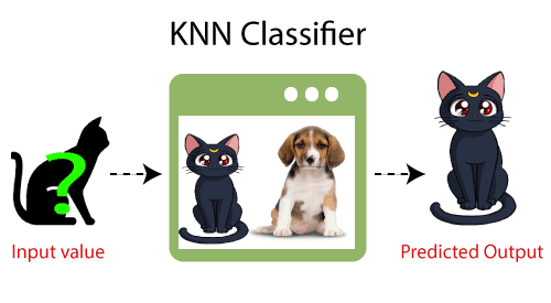
Why do we need a K-NN Algorithm?

Suppose there are two categories, i.e., Category A and Category B, and we have a new data point x1, so this data point will lie in which of these categories. To solve this type of problem, we need a K-NN algorithm. With the help of K-NN, we can easily identify the category or class of a particular dataset. Consider the below diagram:

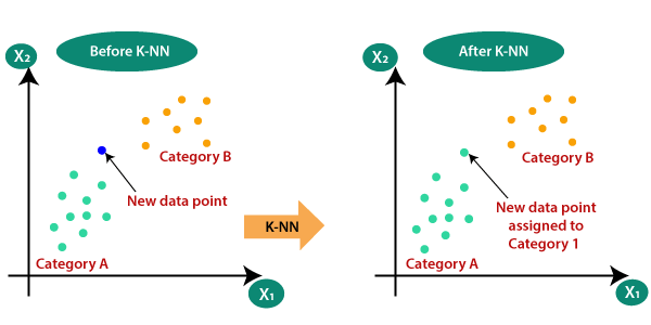
How does K-NN work?

The K-NN working can be explained on the basis of the below algorithm:

• Step-1: Select the number K of the neighbors
• Step-2: Calculate the Euclidean distance of K number of neighbors
• Step-3: Take the K nearest neighbors as per the calculated Euclidean distance.
• Step-4: Among these k neighbors, count the number of the data points in each category.
• Step-5: Assign the new data points to that category for which the number of the neighbor is maximum.
• Step-6: Our model is ready.

Suppose we have a new data point and we need to put it in the required category. Consider the below image:

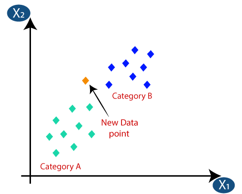
• Firstly, we will choose the number of neighbors, so we will choose the k=5.
• Next, we will calculate the Euclidean distance between the data points. The Euclidean distance is the distance between two points, which we have already studied in geometry. It can be calculated as:

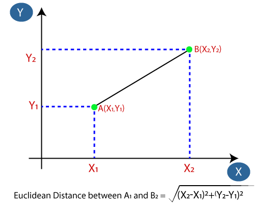
• By calculating the Euclidean distance we got the nearest neighbors, as three nearest neighbors in category A and two nearest neighbors in category B. Consider the below image:

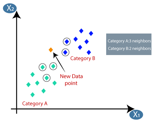
• As we can see the 3 nearest neighbors are from category A, hence this new data point must belong to category A.

How to select the value of K in the K-NN Algorithm?

Below are some points to remember while selecting the value of K in the K-NN algorithm:

• There is no particular way to determine the best value for "K", so we need to try some values to find the best out of them. The most preferred value for K is 5.
• A very low value for K such as K=1 or K=2, can be noisy and lead to the effects of outliers in the model.
• Large values for K are good, but it may find some difficulties.

Advantages of KNN Algorithm:

• It is simple to implement.
• It is robust to the noisy training data
• It can be more effective if the training data is large.

Disadvantages of KNN Algorithm:

• Always needs to determine the value of K which may be complex some time.
• The computation cost is high because of calculating the distance between the data points for all the training samples.

Python implementation of the KNN algorithm

To do the Python implementation of the K-NN algorithm, we will use the same problem and dataset which we have used in Logistic Regression. But here we will improve the performance of the model. Below is the problem description:

Problem for K-NN Algorithm: There is a Car manufacturer company that has manufactured a new SUV car. The company wants to give the ads to the users who are interested in buying that SUV. So for this problem, we have a dataset that contains multiple user's information through the social network. The dataset contains lots of information but the Estimated Salary and Age we will consider for the independent variable and the Purchased variable is for the dependent variable. Below is the dataset:

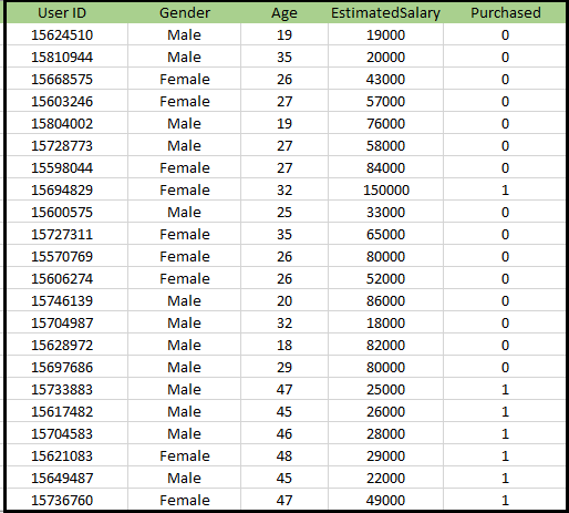
Steps to implement the K-NN algorithm:

• Data Pre-processing step
• Fitting the K-NN algorithm to the Training set
• Predicting the test result
• Test accuracy of the result(Creation of Confusion matrix)
• Visualizing the test set result.

Data Pre-Processing Step:

The Data Pre-processing step will remain exactly the same as Logistic Regression. Below is the code for it:

1. # importing libraries  
2. import numpy as nm  
3. import matplotlib.pyplot as mtp  
4. import pandas as pd  
5.   
6. #importing datasets  
7. data_set= pd.read_csv('user_data.csv')  
8.   
9. #Extracting Independent and dependent Variable  
10. x= data_set.iloc[:, [2,3]].values  
11. y= data_set.iloc[:, 4].values  
12.   
13. # Splitting the dataset into training and test set.  
14. from sklearn.model_selection import train_test_split  
15. x_train, x_test, y_train, y_test= train_test_split(x, y, test_size= 0.25, random_state=0)  
16.   
17. #feature Scaling  
18. from sklearn.preprocessing import StandardScaler    
19. st_x= StandardScaler()    
20. x_train= st_x.fit_transform(x_train)    
21. x_test= st_x.transform(x_test)  

By executing the above code, our dataset is imported to our program and well pre-processed. After feature scaling our test dataset will look like:

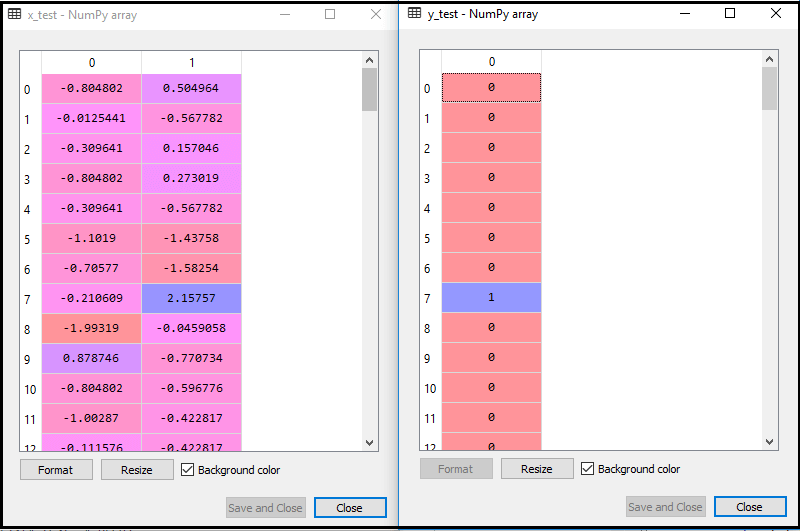
From the above output image, we can see that our data is successfully scaled.

• Fitting K-NN classifier to the Training data:
  Now we will fit the K-NN classifier to the training data. To do this we will import the KNeighborsClassifier class of Sklearn Neighbors library. After importing the class, we will create the Classifier object of the class. The Parameter of this class will be
  • n_neighbors: To define the required neighbors of the algorithm. Usually, it takes 5.
  • metric='minkowski': This is the default parameter and it decides the distance between the points.
  • p=2: It is equivalent to the standard Euclidean metric.
  And then we will fit the classifier to the training data. Below is the code for it:

1. #Fitting K-NN classifier to the training set  
2. from sklearn.neighbors import KNeighborsClassifier  
3. classifier= KNeighborsClassifier(n_neighbors=5, metric='minkowski', p=2 )  
4. classifier.fit(x_train, y_train)  

Output: By executing the above code, we will get the output as:

Out[10]: 
KNeighborsClassifier(algorithm='auto', leaf_size=30, metric='minkowski',
                     metric_params=None, n_jobs=None, n_neighbors=5, p=2,
                     weights='uniform')

• Predicting the Test Result: To predict the test set result, we will create a y_pred vector as we did in Logistic Regression. Below is the code for it:

1. #Predicting the test set result  
2. y_pred= classifier.predict(x_test)  

Output:

The output for the above code will be:

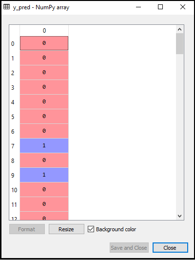
• Creating the Confusion Matrix:
  Now we will create the Confusion Matrix for our K-NN model to see the accuracy of the classifier. Below is the code for it:

1. #Creating the Confusion matrix  
2.     from sklearn.metrics import confusion_matrix  
3.     cm= confusion_matrix(y_test, y_pred)  

In above code, we have imported the confusion_matrix function and called it using the variable cm.

Output: By executing the above code, we will get the matrix as below:

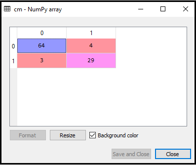
In the above image, we can see there are 64+29= 93 correct predictions and 3+4= 7 incorrect predictions, whereas, in Logistic Regression, there were 11 incorrect predictions. So we can say that the performance of the model is improved by using the K-NN algorithm.

• Visualizing the Training set result:
  Now, we will visualize the training set result for K-NN model. The code will remain same as we did in Logistic Regression, except the name of the graph. Below is the code for it:

1. #Visulaizing the trianing set result  
2. from matplotlib.colors import ListedColormap  
3. x_set, y_set = x_train, y_train  
4. x1, x2 = nm.meshgrid(nm.arange(start = x_set[:, 0].min() - 1, stop = x_set[:, 0].max() + 1, step  =0.01),  
5. nm.arange(start = x_set[:, 1].min() - 1, stop = x_set[:, 1].max() + 1, step = 0.01))  
6. mtp.contourf(x1, x2, classifier.predict(nm.array([x1.ravel(), x2.ravel()]).T).reshape(x1.shape),  
7. alpha = 0.75, cmap = ListedColormap(('red','green' )))  
8. mtp.xlim(x1.min(), x1.max())  
9. mtp.ylim(x2.min(), x2.max())  
10. for i, j in enumerate(nm.unique(y_set)):  
11.     mtp.scatter(x_set[y_set == j, 0], x_set[y_set == j, 1],  
12.         c = ListedColormap(('red', 'green'))(i), label = j)  
13. mtp.title('K-NN Algorithm (Training set)')  
14. mtp.xlabel('Age')  
15. mtp.ylabel('Estimated Salary')  
16. mtp.legend()  
17. mtp.show()  

Output:

By executing the above code, we will get the below graph:

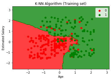
The output graph is different from the graph which we have occurred in Logistic Regression. It can be understood in the below points:

• As we can see the graph is showing the red point and green points. The green points are for Purchased(1) and Red Points for not Purchased(0) variable.
• The graph is showing an irregular boundary instead of showing any straight line or any curve because it is a K-NN algorithm, i.e., finding the nearest neighbor.
• The graph has classified users in the correct categories as most of the users who didn't buy the SUV are in the red region and users who bought the SUV are in the green region.
• The graph is showing good result but still, there are some green points in the red region and red points in the green region. But this is no big issue as by doing this model is prevented from overfitting issues.
• Hence our model is well trained.
• Visualizing the Test set result:
  After the training of the model, we will now test the result by putting a new dataset, i.e., Test dataset. Code remains the same except some minor changes: such as x_train and y_train will be replaced by x_test and y_test.
  Below is the code for it:

1. #Visualizing the test set result  
2. from matplotlib.colors import ListedColormap  
3. x_set, y_set = x_test, y_test  
4. x1, x2 = nm.meshgrid(nm.arange(start = x_set[:, 0].min() - 1, stop = x_set[:, 0].max() + 1, step  =0.01),  
5. nm.arange(start = x_set[:, 1].min() - 1, stop = x_set[:, 1].max() + 1, step = 0.01))  
6. mtp.contourf(x1, x2, classifier.predict(nm.array([x1.ravel(), x2.ravel()]).T).reshape(x1.shape),  
7. alpha = 0.75, cmap = ListedColormap(('red','green' )))  
8. mtp.xlim(x1.min(), x1.max())  
9. mtp.ylim(x2.min(), x2.max())  
10. for i, j in enumerate(nm.unique(y_set)):  
11.     mtp.scatter(x_set[y_set == j, 0], x_set[y_set == j, 1],  
12.         c = ListedColormap(('red', 'green'))(i), label = j)  
13. mtp.title('K-NN algorithm(Test set)')  
14. mtp.xlabel('Age')  
15. mtp.ylabel('Estimated Salary')  
16. mtp.legend()  
17. mtp.show()  

Output:

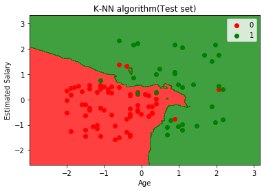
The above graph is showing the output for the test data set. As we can see in the graph, the predicted output is well good as most of the red points are in the red region and most of the green points are in the green region.

Locally Weighted Linear Regression

Within the field of machine learning and regression analysis, Locally Weighted Linear Regression (LWLR) emerges as a notable approach that bolsters predictive accuracy through the integration of local adaptation. In contrast to conventional linear regression models, which presume a universal correlation among variables, LWLR acknowledges the significance of localized patterns and relationships present in the data. In the subsequent discourse, we embark on an exploration of the fundamental principles, diverse applications, and inherent advantages offered by Locally Weighted Linear Regression. Our aim is to shed light on its exceptional capacity to amplify predictive prowess and furnish intricate understandings of intricate datasets.

Fundamentally, LWLR manifests as a non-parametric regression algorithm that discerns the connection between a dependent variable and several independent variables. Notably, LWLR's distinctiveness emanates from its dynamic adaptability, which empowers it to bestow distinct weights upon individual data points contingent on their proximity to the target point under prediction. In essence, this algorithm accords greater significance to proximate data points, deeming them as more influential contributors in the prediction process.

Principles of Locally Weighted Linear Regression

LWLR functions on the premise that the association between the dependent and independent variables adheres to linearity; however, this relationship is allowed to exhibit variability across distinct sections within the dataset. This is achieved by employing an individual linear regression model for each prediction, employing a weighted least squares technique. The determination of weights is carried out through a kernel function, which bestows elevated weights upon data points in close proximity to the target point and diminishes the weights for those that are farther away.

Applications of Locally Weighted Linear Regression

• Time Series Analysis: LWLR is particularly useful in time series analysis, where the relationship between variables may change over time. By adapting to the local patterns and trends, LWLR can capture the dynamics of time-varying data and make accurate predictions.
• Anomaly Detection: LWLR can be employed for anomaly detection in various domains, such as fraud detection or network intrusion detection. By identifying deviations from the expected patterns in a localized manner, LWLR helps detect abnormal behavior that may go unnoticed using traditional regression models.
• Robotics and Control Systems: In robotics and control systems, LWLR can be utilized to model and predict the behavior of complex systems. By adapting to local conditions and variations, LWLR enables precise control and decision-making in dynamic environments.

Benefits of Locally Weighted Linear Regression

• Improved Predictive Accuracy: By considering local patterns and relationships, LWLR can capture subtle nuances in the data that might be overlooked by global regression models. This results in more accurate predictions and better model performance.
• Flexibility and Adaptability: LWLR can adapt to different regions of the dataset, making it suitable for complex and non-linear relationships. It offers flexibility in capturing local variations, allowing for more nuanced analysis and insights.
• Interpretable Results: Despite its adaptive nature, LWLR still provides interpretable results. The localized models offer insights into the relationships between variables within specific regions of the data, aiding in the understanding of complex phenomena.

Radial Basis Function Kernel – Machine Learning

Radial Basis Kernel is a kernel function that is used in machine learning to find a non-linear classifier or regression line.

What is Kernel Function?
Kernel Function is used to transform n-dimensional input to m-dimensional input, where m is much higher than n then find the dot product in higher dimensional efficiently. The main idea to use kernel is: A linear classifier or regression curve in higher dimensions becomes a Non-linear classifier or regression curve in lower dimensions.

Mathematical Definition of Radial Basis Kernel:

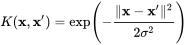
Radial Basis Kernel

where x, x’ are vector point in any fixed dimensional space.
But if we expand the above exponential expression, It will go upto infinite power of x and x’, as expansion of ex contains infinite terms upto infinite power of x hence it involves terms upto infinite powers in infinite dimension.
If we apply any of the algorithms like perceptron Algorithm or linear regression on this kernel, actually we would be applying our algorithm to new infinite-dimensional datapoint we have created. Hence it will give a hyperplane in infinite dimensions, which will give a very strong non-linear classifier or regression curve after returning to our original dimensions.

polynomial of infinite power

So, Although we are applying linear classifier/regression it will give a non-linear classifier or regression line, that will be a polynomial of infinite power. And being a polynomial of infinite power, Radial Basis kernel is a very powerful kernel, which can give a curve fitting any complex dataset.

Why Radial Basis Kernel Is much powerful?
The main motive of the kernel is to do calculations in any d-dimensional space where d > 1, so that we can get a quadratic, cubic or any polynomial equation of large degree for our classification/regression line. Since Radial basis kernel uses exponent and as we know the expansion of e^x gives a polynomial equation of infinite power, so using this kernel, we make our regression/classification line infinitely powerful too.
 
Some Complex Dataset Fitted Using RBF Kernel easily: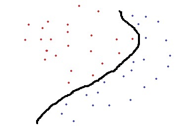


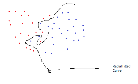
References:

• Radial Basis Kernel
• Kernel Function

Whether you're preparing for your first job interview or aiming to upskill in this ever-evolving tech landscape, GeeksforGeeks Courses are your key to success. We provide top-quality content at affordable prices, all geared towards accelerating your growth in a time-bound manner.

ML | Case Based Reasoning (CBR) Classifier

As we know Nearest Neighbour classifiers stores training tuples as points in Euclidean space. But Case-Based Reasoning classifiers (CBR) use a database of problem solutions to solve new problems. It stores the tuples or cases for problem-solving as complex symbolic descriptions. How CBR works? When a new case arises to classify, a Case-based Reasoner(CBR) will first check if an identical training case exists. If one is found, then the accompanying solution to that case is returned. If no identical case is found, then the CBR will search for training cases having components that are similar to those of the new case. Conceptually, these training cases may be considered as neighbours of the new case. If cases are represented as graphs, this involves searching for subgraphs that are similar to subgraphs within the new case. The CBR tries to combine the solutions of the neighbouring training cases to propose a solution for the new case. If compatibilities arise with the individual solutions, then backtracking to search for other solutions may be necessary. The CBR may employ background knowledge and problem-solving strategies to propose a feasible solution. Applications of CBR includes: 

1. Problem resolution for customer service help desks, where cases describe product-related diagnostic problems.
2. It is also applied to areas such as engineering and law, where cases are either technical designs or legal rulings, respectively.
3. Medical educations, where patient case histories and treatments are used to help diagnose and treat new patients.

Challenges with CBR

• Finding a good similarity metric (eg for matching subgraphs) and suitable methods for combining solutions.
• Selecting salient features for indexing training cases and the development of efficient indexing techniques.

CBR becomes more intelligent as the number of the trade-off between accuracy and efficiency evolves as the number of stored cases becomes very large. But after a certain point, the system’s efficiency will suffer as the time required to search for and process relevant cases increases.

Lazy Learning vs Eager Learning Algorithms in Machine Learning

Introduction

In machine learning, it is essential to understand the algorithm’s working principle and primary classification of the same for avoiding misconceptions and other errors related to the same. There are mainly two types of machine learning algorithms, lazy and eager learning algorithms, based on their training style and other principles. A proper machine learning algorithm should be selected according to the problem statement for a better-performing model.

This article will discuss the lazy and eager learning algorithms with their core intuition, working mechanisms, advantages, and disadvantages. We will also discuss the best-fit model selection according to the data type and requirements of the model. These concepts will help understand the algorithm’s classification better and help understand some common and must-know properties of both types.

Learning Objectives

After going through this article, you will learn the following:

1. The core idea of lazy learning and eager learning algorithms
2. How the lazy and eager learning algorithms work?
3. Difference between both the techniques

This article was published as a part of the Data Science Blogathon.

Table of contents

• What is Eager Learning Algorithm?
• How Does Eager Learning Algorithm Work?
• Lazy vs. Eager Learning Algorithms: The Difference
• Which One is Best for You?
• Conclusion
• Frequently Asked Questions

What is a Lazy Learning Algorithm?

In traditional machine learning, algorithms acquire data, train on it, and produce a trained model capable of predicting unseen datasets with a certain level of accuracy. However, lazy learning algorithms introduce a distinct approach.

Lazy learning algorithms maintain the same underlying mechanism as traditional algorithms but alter how they handle data. During the training phase of lazy learning, the algorithm accepts the data as input but refrains from actively training on it. Instead, it stores the data for later use. The actual model training occurs during the prediction phase.

One prominent example of a lazy learning algorithm is the K-nearest neighbors (KNN) algorithm. KNN stores the data during training and applies its working mechanism when it’s time for prediction or testing.

How Does Lazy Learning Algorithm Work?

Lazy learning algorithms are also known as lazy evaluation algorithms because they evaluate data in a very lazy manner. To illustrate, let’s consider the KNN algorithm as an example. When building a model using KNN, the algorithm accepts and stores the dataset during the training and fitting phase, essentially doing nothing with it.

However, when the testing phase arrives and you request a prediction for a specific data point, the KNN algorithm springs into action. It calculates the nearest neighbors of the given data point based on its working mechanism and returns the predicted output.

It’s essential to note that the training phase for lazy learning algorithms is notably faster since they merely store the data. Conversely, the heavy lifting, involving all the calculations, takes place during the testing phase, making predictions slower and more time-consuming.

What is Eager Learning Algorithm?

Eager learning algorithms are traditional machine learning methods that process data during the training phase. These algorithms build a model based on the provided training data and use this model to make predictions during the prediction phase. Examples of eager learning algorithms include Linear Regression, Logistic Regression, Support Vector Machines, Decision Trees, and Artificial Neural Networks.

How Does Eager Learning Algorithm Work?

Eager learning algorithms take the training data as input and apply various functions and techniques specific to the algorithm during the training phase. For instance, using linear regression for model building processes the data during training, resulting in a trained and knowledgeable model. During the prediction phase, when you request predictions for new data points, the model provides instant results based on training and learning from the initial data. While eager learning algorithms have slower training processes, they offer faster predictions than lazy learning algorithms.

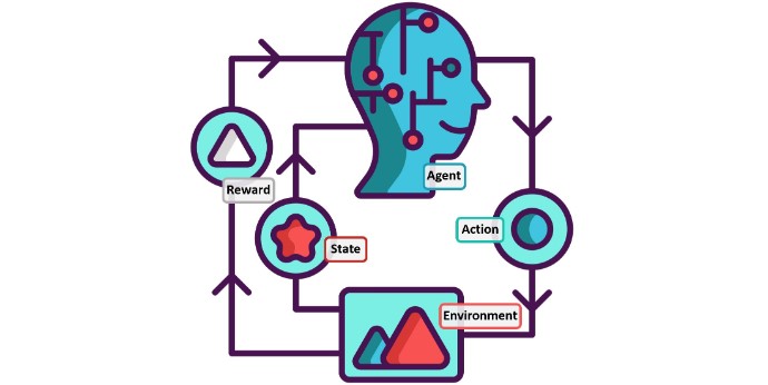
Lazy vs. Eager Learning Algorithms: The Difference

Property	Lazy Learning	Eager Learning
Training Speed	Fast, stores the data while training	Slow, Tries to learn from data while training
Prediction Speed	Too Slow tries to apply functions and learnings in the prediction stage	Faster, predicts very fast as there are pre-defined functions
Learning Scope	Medium, it can learn from data while training	Medium, it can learn from data while testing
Pre Calculated Algorithm	Absent, calculations are done while the testing phase	At present, here calculations are already done in the training phase
Example	KNN	Linear Regression

Which One is Best for You?

After this whole discussion, a question might come to your mind which approach is better and which should be used when?

The answer to this question is in only two words: situation based. As we can not control our data with the algorithm and we cannot changes, we can change the algorithm as per the data and its variations, and that is where the answer to this question lies.

Everything depends on the type of data, its patterns, what kind of model you want, and your requirements. Sometimes, it is essential to train the algorithm faster in an emergency; the lazy learning approach is reasonable. Sometimes it is okay for us to train the model for a longer time to make it faster while prediction than the enthusiastic learning approach is reasonable.

In some of the datasets, the behavior of the data matches very correctly to some of the lazy learning approaches, and you also want a fast predictor model; in such cases, you can use sluggish learning methods and apply some other techniques or tune the algorithm in such a way that model becomes less complex and takes less time to predict.

Conclusion

In this article, we discussed the lazy and eager learning algorithms in machine learning with core intuition and ideas behind them with suitable examples. We also discussed an approach for selecting the best-fit algorithm according to the problem statement. This will help one to identify the algorithm, classify them, and use them correctly.

Some of the Key Takeaways from this article are:

• Lazy learning algorithms are types of algorithms that store the data while training and preprocessing it during the testing phase.
• Lazy learning algorithms take a shorter time for training and a longer time for predicting.
• The eager learning algorithm processes the data while the training phase is only.
• Eager learning algorithms are faster than lazy learning algorithms for predicting data observations.
• A proper approach should be selected according to the model’s data type and requirements.