
What Is An Algorithm? Definition, Types, Characteristics
What is an Algorithm?
An algorithm is a set of commands that must be followed for a
computer to perform calculations or other problem-solving operations.According
to its formal definition, an algorithm is a finite set of instructions carried
out in a specific order to perform a particular task. It is not the entire
program or code; it is simple logic to a problem represented as an informal
description in the form of a flowchart or pseudocode.

Problem: A
problem can be defined as a real-world problem or real-world instance problem
for which you need to develop a program or set of instructions. An algorithm is
a set of instructions.
Algorithm:
An algorithm is defined as a step-by-step process that will be designed for a
problem.
Input: After
designing an algorithm, the algorithm is given the necessary and desired
inputs.
Processing
unit: The input will be passed to the processing unit, producing the desired
output.
Output: The
outcome or result of the program is referred to as the output.
After defining what an algorithm is, you will now look at
algorithm characteristics.
How do Algorithms Work?
Algorithms are step-by-step procedures designed to solve
specific problems and perform tasks efficiently in the realm of computer
science and mathematics. These powerful sets of instructions form the backbone
of modern technology and govern everything from web searches to artificial
intelligence. Here's how algorithms work:
Input: Algorithms take input data, which can be in various
formats, such as numbers, text, or images.
Processing: The algorithm processes the input data through a
series of logical and mathematical operations, manipulating and transforming it
as needed.
Output: After the processing is complete, the algorithm
produces an output, which could be a result, a decision, or some other
meaningful information.
Efficiency: A key aspect of algorithms is their efficiency,
aiming to accomplish tasks quickly and with minimal resources.
Optimization: Algorithm designers constantly seek ways to
optimize their algorithms, making them faster and more reliable.
Implementation: Algorithms are implemented in various
programming languages, enabling computers to execute them and produce desired
outcomes.
What is the Need for Algorithms?
You require algorithms for the following reasons:
Scalability
It aids in your understanding of scalability. When you have a
sizable real-world problem, you must break it down into small steps to analyze
it quickly.
Performance
The real world is challenging to break down into smaller
steps. If a problem can be easily divided into smaller steps, it indicates that
the problem is feasible.
After understanding what is an algorithm, why you need an
algorithm, you will look at how to write one using an example.
Types of Algorithms
Brute Force Algorithm: A straightforward approach that
exhaustively tries all possible solutions, suitable for small problem instances
but may become impractical for larger ones due to its high time complexity.
Recursive Algorithm: A method that breaks a problem into
smaller, similar subproblems and repeatedly applies itself to solve them until
reaching a base case, making it effective for tasks with recursive structures.
Encryption Algorithm: Utilized to transform data into a
secure, unreadable form using cryptographic techniques, ensuring
confidentiality and privacy in digital communications and transactions.
Backtracking Algorithm: A trial-and-error technique used to
explore potential solutions by undoing choices when they lead to an incorrect
outcome, commonly employed in puzzles and optimization problems.
Searching Algorithm: Designed to find a specific target
within a dataset, enabling efficient retrieval of information from sorted or
unsorted collections.
Sorting Algorithm: Aimed at arranging elements in a specific
order, like numerical or alphabetical, to enhance data organization and
retrieval.
Hashing Algorithm: Converts data into a fixed-size hash
value, enabling rapid data access and retrieval in hash tables, commonly used
in databases and password storage.
Divide and Conquer Algorithm: Breaks a complex problem into
smaller subproblems, solves them independently, and then combines their
solutions to address the original problem effectively.
Greedy Algorithm: Makes locally optimal choices at each step
in the hope of finding a global optimum, useful for optimization problems but
may not always lead to the best solution.
Dynamic Programming Algorithm:
Stores and reuses intermediate results to avoid redundant computations,
enhancing the efficiency of solving complex problems.
Randomized Algorithm: Utilizes randomness in its steps to
achieve a solution, often used in situations where an approximate or
probabilistic answer suffices.
How to Write an
Algorithm?
There are no
well-defined standards for writing algorithms. It is, however, a problem that
is resource-dependent. Algorithms are never written with a specific programming
language in mind.
As you all
know, basic code constructs such
as loops like do, for, while, all programming
languages share flow control such as if-else, and so on. An
algorithm can be written using these common constructs.
Algorithms
are typically written in a step-by-step fashion, but this is not always the
case. Algorithm writing is a process that occurs after the problem domain has
been well-defined. That is, you must be aware of the problem domain for which
you are developing a solution.
Example
Now, use an example to learn how to write algorithms.
Problem: Create an algorithm that multiplies two numbers and
displays the output.
|
Step 1 − Start Step 2 − declare three
integers x, y & z Step 3 − define values of x
& y Step 4 − multiply values of
x & y Step 5 − store result of
step 4 to z Step 6 − print z Step 7 − Stop |
Algorithms instruct programmers on how to
write code. In addition, the algorithm can be written as:
|
Step 1 − Start mul Step 2 − get values of x
& y Step 3 − z ← x * y Step 4 − display z Step 5 − Stop |
In algorithm design and analysis, the second method is
typically used to describe an algorithm. It allows the analyst to analyze the
algorithm while ignoring all unwanted definitions easily. They can see which
operations are being used and how the process is progressing. It is optional to
write step numbers. To solve a given problem, you create an algorithm. A
problem can be solved in a variety of ways.
As a result, many solution algorithms for a given problem can
be derived. The following step is to evaluate the proposed solution algorithms
and implement the most appropriate solution.
As you progress through this "what is an Algorithm"
tutorial, you will learn about some of the components of an algorithm.
Factors of an Algorithm
The following are the factors to consider when designing an
algorithm:
Modularity:
This feature was perfectly designed for the algorithm if you are given a
problem and break it down into small-small modules or small-small steps, which
is a basic definition of an algorithm.
Correctness:
An algorithm's correctness is defined as when the given inputs produce the
desired output, indicating that the algorithm was designed correctly. An
algorithm's analysis has been completed correctly.
Maintainability:
It means that the algorithm should be designed in a straightforward, structured
way so that when you redefine the algorithm, no significant changes are made to
the algorithm.
Functionality:
It takes into account various logical steps to solve a real-world problem.
Robustness:
Robustness refers to an algorithm's ability to define your problem clearly.
User-friendly:
If the algorithm is difficult to understand, the designer will not explain it
to the programmer.
Simplicity:
If an algorithm is simple, it is simple to understand.
Extensibility:
Your algorithm should be extensible if another algorithm designer or programmer
wants to use it.
You will now see why an algorithm is so essential after understanding some of its components.
Qualities of a Good Algorithm
Efficiency:
A good algorithm should perform its task quickly and use minimal resources.
Correctness:
It must produce the correct and accurate output for all valid inputs.
Clarity: The
algorithm should be easy to understand and comprehend, making it maintainable
and modifiable.
Scalability:
It should handle larger data sets and problem sizes without a significant
decrease in performance.
Reliability:
The algorithm should consistently deliver correct results under different
conditions and environments.
Optimality:
Striving for the most efficient solution within the given problem constraints.
Robustness:
Capable of handling unexpected inputs or errors gracefully without crashing.
Adaptability:
Ideally, it can be applied to a range of related problems with minimal
adjustments.
Simplicity:
Keeping the algorithm as simple as possible while meeting its requirements,
avoiding unnecessary complexity.
The Complexity of an Algorithm
The algorithm's performance can be measured in two ways:
Time Complexity
The amount of time required to complete an algorithm's
execution is called time complexity. The
big O notation is used to represent an algorithm's time complexity. The
asymptotic notation for describing time complexity, in this case, is big O
notation. The time complexity is calculated primarily by counting the number of
steps required to complete the execution. Let us look at an example of time
complexity.
|
mul = 1; // Suppose you have to
calculate the multiplication of n numbers. for i=1 to n mul = mul *1; // when the loop ends, then
mul holds the multiplication of the n numbers return mul; |
The time complexity of the loop statement in the preceding
code is at least n, and as the value of n escalates, so does the time
complexity. While the code's complexity, i.e., returns mul, will be constant
because its value is not dependent on the importance of n and will provide the
result in a single step. The worst-time complexity is generally considered
because it is the maximum time required for any given input size.
Space Complexity
The amount of space an algorithm requires to solve a problem
and produce an output is called its space complexity. Space complexity, like
time complexity, is expressed in big O notation.
The space is required for an algorithm for the following
reasons:
To store
program instructions.
To store
track of constant values.
To store
track of variable values.
To store
track of function calls, jumping statements, and so on.
Space Complexity = Auxiliary Space + Input Size
Finally after understanding what is an algorithm, its
analysis and approches, you will look at different types of algorithms.
Advantage and Disadvantages of Algorithms
Advantages of Algorithms:
Efficiency:
Algorithms streamline processes, leading to faster and more optimized
solutions.
Reproducibility:
They yield consistent results when provided with the same inputs.
Problem-solving:
Algorithms offer systematic approaches to tackle complex problems effectively.
Scalability:
Many algorithms can handle larger datasets and scale with increasing input
sizes.
Automation:
They enable automation of tasks, reducing the need for manual intervention.
Disadvantages of Algorithms:
Complexity:
Developing sophisticated algorithms can be challenging and time-consuming.
Limitations:
Some problems may not have efficient algorithms, leading to suboptimal
solutions.
Resource
Intensive: Certain algorithms may require significant computational resources.
Inaccuracy:
Inappropriate algorithm design or implementation can result in incorrect
outputs.
Maintenance:
As technology evolves, algorithms may require updates to stay relevant and
effective.
Randomized Algorithms
Introduction
As we all
know, algorithms are step-by-step procedure that is used to solve
problems or to do some calculations. While most algorithms use a defined set of
rules, we can introduce some randomness in their logic to make them into
randomized algorithms.
Randomized Algorithms use
some randomness in their logic to improve efficiency, time complexity, or maybe
the total memory used. Let us dig deeper into the blog; Randomized Algorithms to know more.
What is Randomized Algorithms?
Randomized
algorithms are a class of algorithms in computer science that use randomness or
randomness in combination with deterministic steps to solve computational
problems. These algorithms introduce randomness intentionally into their
calculations to achieve specific goals, such as improving efficiency or
increasing the likelihood of finding a correct solution.
Randomized
algorithms are particularly useful in situations where finding an exact
solution to a problem is computationally expensive or impractical. They often
provide approximate solutions with a controlled level of error. Some common
applications of randomized algorithms include:
A Las
Vegas or a Monte Carlo are the two most frequent algorithms to build randomized
algorithms. We will see many things about them in the later section of the
blog.
Need for
Randomized Algorithms
Several
questions must arise in your brain, like why do we even need to add randomness
to our logic? What is the requirement of doing so? For example, if we have a
quick sort that works fine, why do we add randomness to its logic?
This
section of the blog will give you a few advantages of Randomized algorithms
that will help to clear most of your doubts regarding the need for Randomized
algorithms.

1. Improved Efficiency: Adding randomness to
the logic of an Algorithm might reduce the likelihood of that worst-case
scenario happening, thus increasing its efficiency.
2. Complex Problems can be Handled Effectively:
Randomized algorithms are suitable for difficult situations because they manage
complex issues that are difficult to solve deterministically by providing
approximate solutions or many other techniques.
3. Worst-Case Scenarios can be avoided: we
have already discussed this advantage of randomized algorithms. Take the
example of the quick sort; introducing random pivot selection in the logic can
reduce the probability of falling into the worst-case scenario of the
algorithm, improving the overall time complexity.
4. Cryptography: In cryptography, randomness is essential for
creating secure keys, ensuring unpredictable results, and protecting against
attacks. To increase security, randomized algorithms are used in random number
generation, encryption techniques, and cryptographic protocols.
Looking
at the above advantages of randomized algorithms we can safely say that
randomized algorithms not only increase the efficiency of the program but also
sometimes increase the security of the program.
Classification
of Randomized Algorithms
Randomized
algorithms can be roughly grouped into numerous categories based on their
properties and applications. Here are two broadly classified categories of
randomized algorithms.

1. Monte Carlo Algorithms: To approximate numerical
values or solve issues probabilistically, Monte Carlo methods use
randomization. With a certain degree of assurance, they offer an approximate
solution. Example includes, calculating the value of π, resolving optimization
problems, or doing probabilistic simulations.
2. Las Vegas Algorithms: A Las Vegas algorithm
executes in a predetermined period of time. It is predictable that it runs out
of time and doesn't find any solutions, but if it finds one within that window,
it will be precisely correct.
Note: Due to the algorithm's potential
for producing inaccurate results, an algorithm called as amplification is utilized to
increase the likelihood of correctness while degrading runtime. The randomized
algorithm is used numerous times with various random subsamples of the input,
and the results are then compared to achieve amplification.
Let’s
discuss each one of them one by one in the next few sections of this blog.
Monte Carlo Algorithms
The goal
of the Monte Carlo approach
for randomized algorithms is to complete the execution within the allotted time
limit. This method's running time is therefore predictable. For instance, when performing string matching,
Monte Carlo starts the procedure over from the last error it encountered. Thus,
time is saved.
A deterministic algorithm's output is always
anticipated to be right, whereas Monte Carlo techniques can not guarantee this.
These algorithms are typically categorized as either false-biased or true-biased for decision issues. When a false-biased
Monte Carlo algorithm delivers false, it is always correct; likewise, a
true-biased method always yields true.
Technical Example: Approximating π(pi)
The
answer to approximating pi, or the ratio of a circle's circumference to its
diameter, or "pi", provides a famous illustration of a more complex
Monte Carlo process. This approximation problem is so typical that huge banks
and other mathematically demanding businesses ask candidates for programming
positions in interviews about it.
Las Vegas Algorithms
This is a
randomized algorithm that consistently yields the right answer or fails. Still,
it cannot guarantee a time limit because the time complexity depends on the
input. Virtually every search result contains a Las Vegas algorithm. Consider a
Las Vegas algorithm as a problem whose answer, when found, is certain to be the
right one but whose route to that answer may be uncertain.
The
term "Las Vegas" for
this algorithm is credited to mathematician Laszlo Babai, who came up with it
in 1979 simply as a comparison to the much older Monte Carlo algorithm as both
are significant global gaming centers.
Technical Example: Randomized Quicksort
Quicksort is a common Las Vegas
randomized sorting method that uses no additional memory and sorts elements in
place. Since this technique is comparison-based, the worst case will happen
when doing a pairwise comparison, which takes O(n^2) time complexity, where the time needed grows as
a square of the number of digits to be sorted. However, with randomization,
this algorithm's worst-case time complexity can be lowered to O(n log(n)).
If the
pivot element selected at random is the first or final member in the array, the
worst-case scenario for this technique is that it takes O(n^2) time to sort n
digits.
The
anticipated runtime for randomized algorithms, i.e., Quicksort, where the pivot
is selected randomly, and neither the smallest nor largest number in the array
is chosen, is O(n log(n)).
Relation
between Monte-carlo and Las Vegas
By
executing a Las Vegas algorithm for a predetermined amount of time and
producing a random response when it fails to terminate, it can be transformed
into a Monte Carlo algorithm.
Below is the table that shows the relation between
two algorithms.
|
|
Monte Carlo Algorithm |
Las Vegas Algorithm |
|
Correctness |
Probabilistic |
Certain |
|
Running Time |
Certain |
Probabilistic |
Now let
us discuss some frequently Asked Questions on Randomized Algorithm.
Advantages of Randomized Algorithms
Advantages
of randomized algorithms are:
·
Efficiency: They
often provide faster solutions, especially for complex problems.
·
Simplicity: They
can be simpler to implement than deterministic alternatives.
·
Approximate Solutions: Useful
when exact solutions are hard or unnecessary.
·
Probabilistic
Correctness: Offer high probability of correctness, balancing reliability and
speed.
·
Versatility:
Applicable in various fields like computer science, math, and optimization.
·
Parallelism: Easily
parallelizable, making them suitable for modern computing architectures.
·
Privacy: Useful
for ensuring data privacy in scenarios like cryptography.
·
Robustness:
Resilient to variations and uncertainties, valuable in real-world scenarios.
Limitations of Randomized Algorithms
Limitations
of randomized algorithms are:
·
Probabilistic Output: They
provide approximate solutions with a probability of correctness, not guaranteed
accuracy.
·
Analysis Complexity: Evaluating
their performance can be challenging due to randomness.
·
Deterministic
Alternatives: In some cases, deterministic algorithms provide certainty at the
cost of speed.
·
Difficulty in Reproduction: Results
may vary between runs, making them less predictable.
·
Resource Usage: May
consume more memory or time due to random operations.
·
Not Always Suitable: Unsuitable
for tasks requiring exact, reliable results.
·
Complexity: Designing
and analyzing randomized algorithms can be complex.
·
Error Control: Ensuring
the acceptable level of error requires careful consideration.
Divide and Conquer Introduction
Divide and Conquer is an algorithmic pattern. In algorithmic methods, the design is to take a dispute on a huge input, break the input into minor pieces, decide the problem on each of the small pieces, and then merge the piecewise solutions into a global solution. This mechanism of solving the problem is called the Divide & Conquer Strategy.
Divide and Conquer algorithm consists of a dispute using the following three steps.
- Divide the original problem into a set of subproblems.
- Conquer: Solve every subproblem individually, recursively.
- Combine: Put together the solutions of the subproblems to get the solution to the whole problem.
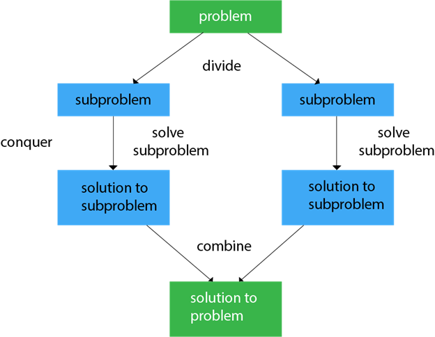
Generally, we can follow the divide-and-conquer approach in a three-step process.
Examples: The specific computer algorithms are based on the Divide & Conquer approach:
- Maximum and Minimum Problem
- Binary Search
- Sorting (merge sort, quick sort)
- Tower of Hanoi.
Fundamental of Divide & Conquer Strategy:
There are two fundamental of Divide & Conquer Strategy:
- Relational Formula
- Stopping Condition
1. Relational Formula: It is the formula that we generate from the given technique. After generation of Formula we apply D&C Strategy, i.e. we break the problem recursively & solve the broken subproblems.
2. Stopping Condition: When we break the problem using Divide & Conquer Strategy, then we need to know that for how much time, we need to apply divide & Conquer. So the condition where the need to stop our recursion steps of D&C is called as Stopping Condition.
Applications of Divide and Conquer Approach:
Following algorithms are based on the concept of the Divide and Conquer Technique:
- Binary Search: The binary search algorithm is a searching algorithm, which is also called a half-interval search or logarithmic search. It works by comparing the target value with the middle element existing in a sorted array. After making the comparison, if the value differs, then the half that cannot contain the target will eventually eliminate, followed by continuing the search on the other half. We will again consider the middle element and compare it with the target value. The process keeps on repeating until the target value is met. If we found the other half to be empty after ending the search, then it can be concluded that the target is not present in the array.
- Quicksort: It is the most efficient sorting algorithm, which is also known as partition-exchange sort. It starts by selecting a pivot value from an array followed by dividing the rest of the array elements into two sub-arrays. The partition is made by comparing each of the elements with the pivot value. It compares whether the element holds a greater value or lesser value than the pivot and then sort the arrays recursively.
- Merge Sort: It is a sorting algorithm that sorts an array by making comparisons. It starts by dividing an array into sub-array and then recursively sorts each of them. After the sorting is done, it merges them back.
- Closest Pair of Points: It is a problem of computational geometry. This algorithm emphasizes finding out the closest pair of points in a metric space, given n points, such that the distance between the pair of points should be minimal.
- Strassen's Algorithm: It is an algorithm for matrix multiplication, which is named after Volker Strassen. It has proven to be much faster than the traditional algorithm when works on large matrices.
- Cooley-Tukey Fast Fourier Transform (FFT) algorithm: The Fast Fourier Transform algorithm is named after J. W. Cooley and John Turkey. It follows the Divide and Conquer Approach and imposes a complexity of O(nlogn).
- Karatsuba algorithm for fast multiplication: It is one of the fastest multiplication algorithms of the traditional time, invented by Anatoly Karatsuba in late 1960 and got published in 1962. It multiplies two n-digit numbers in such a way by reducing it to at most single-digit.
Advantages of Divide and Conquer
- Divide and Conquer tend to successfully solve one of the biggest problems, such as the Tower of Hanoi, a mathematical puzzle. It is challenging to solve complicated problems for which you have no basic idea, but with the help of the divide and conquer approach, it has lessened the effort as it works on dividing the main problem into two halves and then solve them recursively. This algorithm is much faster than other algorithms.
- It efficiently uses cache memory without occupying much space because it solves simple subproblems within the cache memory instead of accessing the slower main memory.
- It is more proficient than that of its counterpart Brute Force technique.
- Since these algorithms inhibit parallelism, it does not involve any modification and is handled by systems incorporating parallel processing.
Disadvantages of Divide and Conquer
- Since most of its algorithms are designed by incorporating recursion, so it necessitates high memory management.
- An explicit stack may overuse the space.
- It may even crash the system if the recursion is performed rigorously greater than the stack present in the CPU.
Binary Search – Data Structure and Algorithm Tutorials
Conditions for when to apply Binary Search in a Data Structure:
To apply Binary Search algorithm:
- The data structure must be sorted.
- Access to any element of the data structure takes constant time.
Binary Search Algorithm:
In this algorithm,
- Divide the search space into two halves by finding the middle index “mid”.
Finding the middle index “mid” in Binary Search Algorithm
- Compare the middle element of the search space with the key.
- If the key is found at middle element, the process is terminated.
- If the key is not found at middle element, choose which half will be used as the next search space.
- If the key is smaller than the middle element, then the left side is used for next search.
- If the key is larger than the middle element, then the right side is used for next search.
- This process is continued until the key is found or the total search space is exhausted.
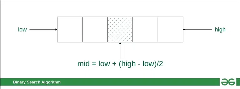
Consider an array arr[] = {2, 5, 8, 12, 16, 23, 38, 56, 72, 91}, and the target = 23.
First Step: Calculate the mid and compare the mid element with the key. If the key is less than mid element, move to left and if it is greater than the mid then move search space to the right.
- Key (i.e., 23) is greater than current mid element (i.e., 16). The search space moves to the right.
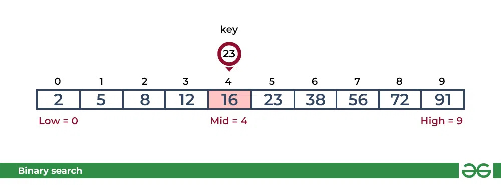
Binary Search Algorithm : Compare key with 16
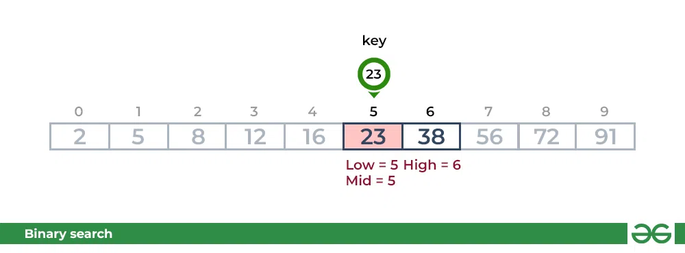
- Key is less than the current mid 56. The search space moves to the left.

Binary Search Algorithm : Compare key with 56
Second Step: If the key matches the value of the mid element, the element is found and stop search.
// C++ program to implement iterative Binary Search
#include <bits/stdc++.h>
using namespace std;
// An iterative binary search function.
int binarySearch(int arr[], int l, int r, int x)
{
while (l <= r) {
int m = l + (r - l) / 2;
// Check if x is present at mid
if (arr[m] == x)
return m;
// If x greater, ignore left half
if (arr[m] < x)
l = m + 1;
// If x is smaller, ignore right half
else
r = m - 1;
}
// If we reach here, then element was not present
return -1;
}
// Driver code
int main(void)
{
int arr[] = { 2, 3, 4, 10, 40 };
int x = 10;
int n = sizeof(arr) / sizeof(arr[0]);
int result = binarySearch(arr, 0, n - 1, x);
(result == -1)
? cout << "Element is not present in array"
: cout << "Element is present at index " << result;
return 0;
}
Element is present at index 3
Finding the maximum and minimum number
// C++ implementation of the above approach
#include <bits/stdc++.h>
using namespace std;
struct Pair {
int min;
int max;
};
Pair getMinMax(int arr[], int n)
{
Pair minmax;
sort(arr, arr + n);
minmax.min = arr[0];
minmax.max = arr[n - 1];
return minmax;
}
int main()
{
int arr[] = { 1000, 11, 445, 1, 330, 3000 };
int arr_size = sizeof(arr) / sizeof(arr[0]);
Pair minmax = getMinMax(arr, arr_size);
cout << "Minimum element is " << minmax.min << endl;
cout << "Maximum element is " << minmax.max << endl;
return 0;
}
Merge Sort – Data Structure and Algorithms
In simple terms, we can say that the process of merge sort is to divide the array into two halves, sort each half, and then merge the sorted halves back together. This process is repeated until the entire array is sorted.
.png)
Merge Sort Algorithm
How does Merge Sort work?
Merge sort is a recursive algorithm that continuously splits the array in half until it cannot be further divided i.e., the array has only one element left (an array with one element is always sorted). Then the sorted subarrays are merged into one sorted array.
// C++ program for Merge Sort
#include <bits/stdc++.h>
using namespace std;
// Merges two subarrays of array[].
// First subarray is arr[begin..mid]
// Second subarray is arr[mid+1..end]
void merge(int array[], int const left, int const mid,
int const right)
{
int const subArrayOne = mid - left + 1;
int const subArrayTwo = right - mid;
// Create temp arrays
auto *leftArray = new int[subArrayOne],
*rightArray = new int[subArrayTwo];
// Copy data to temp arrays leftArray[] and rightArray[]
for (auto i = 0; i < subArrayOne; i++)
leftArray[i] = array[left + i];
for (auto j = 0; j < subArrayTwo; j++)
rightArray[j] = array[mid + 1 + j];
auto indexOfSubArrayOne = 0, indexOfSubArrayTwo = 0;
int indexOfMergedArray = left;
// Merge the temp arrays back into array[left..right]
while (indexOfSubArrayOne < subArrayOne
&& indexOfSubArrayTwo < subArrayTwo) {
if (leftArray[indexOfSubArrayOne]
<= rightArray[indexOfSubArrayTwo]) {
array[indexOfMergedArray]
= leftArray[indexOfSubArrayOne];
indexOfSubArrayOne++;
}
else {
array[indexOfMergedArray]
= rightArray[indexOfSubArrayTwo];
indexOfSubArrayTwo++;
}
indexOfMergedArray++;
}
// Copy the remaining elements of
// left[], if there are any
while (indexOfSubArrayOne < subArrayOne) {
array[indexOfMergedArray]
= leftArray[indexOfSubArrayOne];
indexOfSubArrayOne++;
indexOfMergedArray++;
}
// Copy the remaining elements of
// right[], if there are any
while (indexOfSubArrayTwo < subArrayTwo) {
array[indexOfMergedArray]
= rightArray[indexOfSubArrayTwo];
indexOfSubArrayTwo++;
indexOfMergedArray++;
}
delete[] leftArray;
delete[] rightArray;
}
// begin is for left index and end is right index
// of the sub-array of arr to be sorted
void mergeSort(int array[], int const begin, int const end)
{
if (begin >= end)
return;
int mid = begin + (end - begin) / 2;
mergeSort(array, begin, mid);
mergeSort(array, mid + 1, end);
merge(array, begin, mid, end);
}
// UTILITY FUNCTIONS
// Function to print an array
void printArray(int A[], int size)
{
for (int i = 0; i < size; i++)
cout << A[i] << " ";
cout << endl;
}
// Driver code
int main()
{
int arr[] = { 12, 11, 13, 5, 6, 7 };
int arr_size = sizeof(arr) / sizeof(arr[0]);
cout << "Given array is \n";
printArray(arr, arr_size);
mergeSort(arr, 0, arr_size - 1);
cout << "\nSorted array is \n";
printArray(arr, arr_size);
return 0;
}
Quick sort
// C++ Implementation of the Quick Sort Algorithm.
#include <iostream>
using namespace std;
int partition(int arr[], int start, int end)
{
int pivot = arr[start];
int count = 0;
for (int i = start + 1; i <= end; i++) {
if (arr[i] <= pivot)
count++;
}
// Giving pivot element its correct position
int pivotIndex = start + count;
swap(arr[pivotIndex], arr[start]);
// Sorting left and right parts of the pivot element
int i = start, j = end;
while (i < pivotIndex && j > pivotIndex) {
while (arr[i] <= pivot) {
i++;
}
while (arr[j] > pivot) {
j--;
}
if (i < pivotIndex && j > pivotIndex) {
swap(arr[i++], arr[j--]);
}
}
return pivotIndex;
}
void quickSort(int arr[], int start, int end)
{
// base case
if (start >= end)
return;
// partitioning the array
int p = partition(arr, start, end);
// Sorting the left part
quickSort(arr, start, p - 1);
// Sorting the right part
quickSort(arr, p + 1, end);
}
int main()
{
int arr[] = { 9, 3, 4, 2, 1, 8 };
int n = 6;
quickSort(arr, 0, n - 1);
for (int i = 0; i < n; i++) {
cout << arr[i] << " ";
}
return 0;
}
1 2 3 4 8 9
Selection Sort – Data Structure and Algorithm
The algorithm repeatedly selects the smallest (or largest) element from the unsorted portion of the list and swaps it with the first element of the unsorted part. This process is repeated for the remaining unsorted portion until the entire list is sorted.
How does Selection Sort Algorithm work?
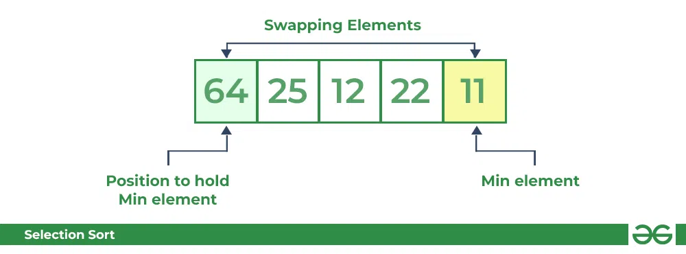
Lets consider the following array as an example: arr[] = {64, 25, 12, 22, 11}
First pass:
- For the first position in the sorted array, the whole array is traversed from index 0 to 4 sequentially. The first position where 64 is stored presently, after traversing whole array it is clear that 11 is the lowest value.
- Thus, replace 64 with 11. After one iteration 11, which happens to be the least value in the array, tends to appear in the first position of the sorted list.
Selection Sort Algorithm | Swapping 1st element with the minimum in array
Second Pass:
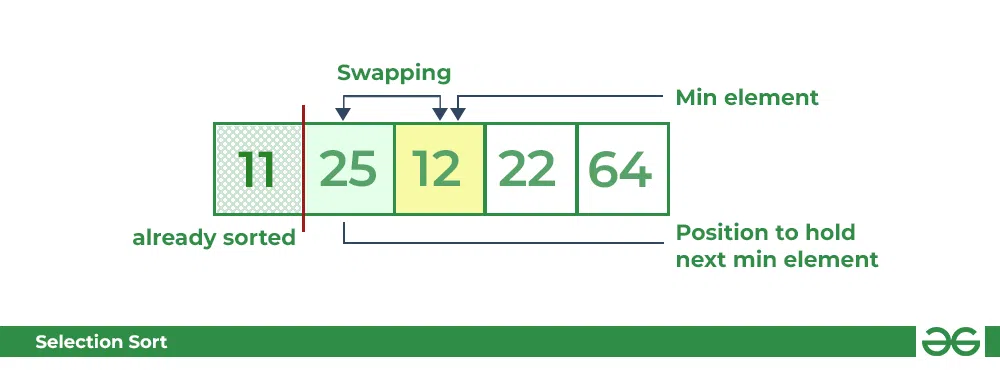
- For the second position, where 25 is present, again traverse the rest of the array in a sequential manner.
- After traversing, we found that 12 is the second lowest value in the array and it should appear at the second place in the array, thus swap these values.
Selection Sort Algorithm | swapping i=1 with the next minimum element
Third Pass:
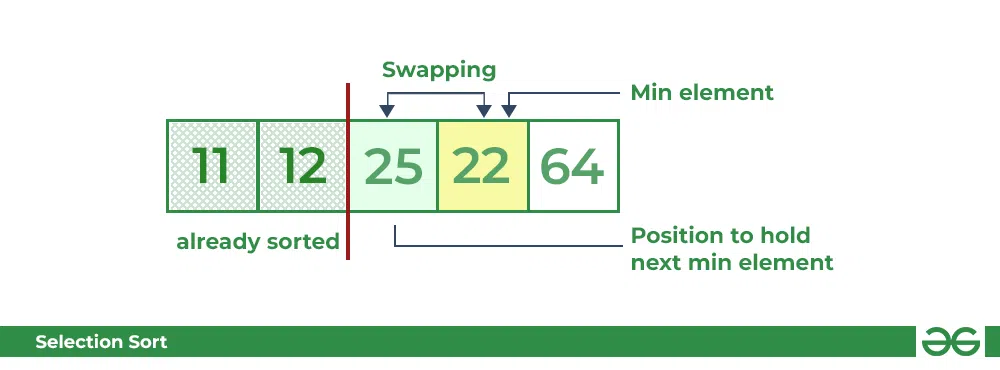
- Now, for third place, where 25 is present again traverse the rest of the array and find the third least value present in the array.
- While traversing, 22 came out to be the third least value and it should appear at the third place in the array, thus swap 22 with element present at third position.
Selection Sort Algorithm | swapping i=2 with the next minimum element
Fourth pass:
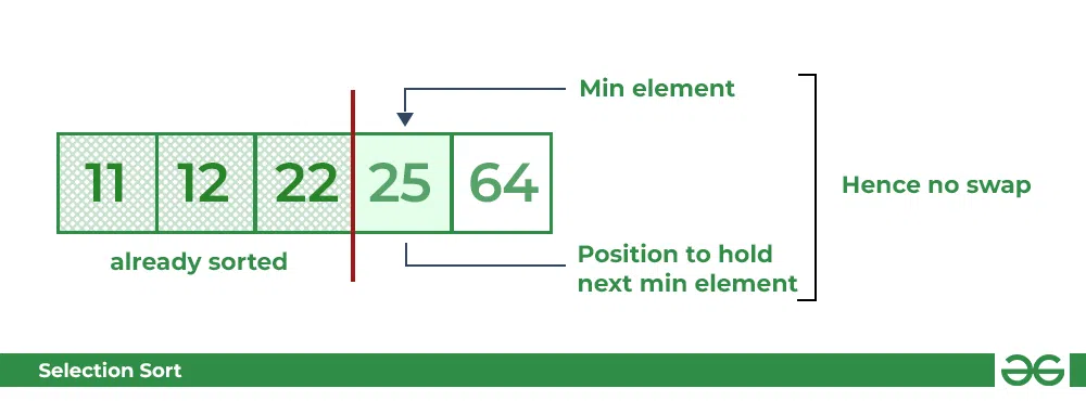
- Similarly, for fourth position traverse the rest of the array and find the fourth least element in the array
- As 25 is the 4th lowest value hence, it will place at the fourth position.
Selection Sort Algorithm | swapping i=3 with the next minimum element
Fifth Pass:
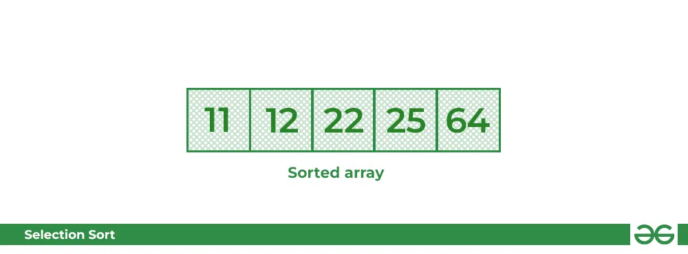
- At last the largest value present in the array automatically get placed at the last position in the array
- The resulted array is the sorted array.
Strassen's matrix multiplication problem#include <bits/stdc++.h> using namespace std; #define ROW_1 4 #define COL_1 4 #define ROW_2 4 #define COL_2 4 void print(string display, vector<vector<int> > matrix, int start_row, int start_column, int end_row, int end_column) { cout << endl << display << " =>" << endl; for (int i = start_row; i <= end_row; i++) { for (int j = start_column; j <= end_column; j++) { cout << setw(10); cout << matrix[i][j]; } cout << endl; } cout << endl; return; } void add_matrix(vector<vector<int> > matrix_A, vector<vector<int> > matrix_B, vector<vector<int> >& matrix_C, int split_index) { for (auto i = 0; i < split_index; i++) for (auto j = 0; j < split_index; j++) matrix_C[i][j] = matrix_A[i][j] + matrix_B[i][j]; } vector<vector<int> > multiply_matrix(vector<vector<int> > matrix_A, vector<vector<int> > matrix_B) { int col_1 = matrix_A[0].size(); int row_1 = matrix_A.size(); int col_2 = matrix_B[0].size(); int row_2 = matrix_B.size(); if (col_1 != row_2) { cout << "\nError: The number of columns in Matrix " "A must be equal to the number of rows in " "Matrix B\n"; return {}; } vector<int> result_matrix_row(col_2, 0); vector<vector<int> > result_matrix(row_1, result_matrix_row); if (col_1 == 1) result_matrix[0][0] = matrix_A[0][0] * matrix_B[0][0]; else { int split_index = col_1 / 2; vector<int> row_vector(split_index, 0); vector<vector<int> > result_matrix_00(split_index, row_vector); vector<vector<int> > result_matrix_01(split_index, row_vector); vector<vector<int> > result_matrix_10(split_index, row_vector); vector<vector<int> > result_matrix_11(split_index, row_vector); vector<vector<int> > a00(split_index, row_vector); vector<vector<int> > a01(split_index, row_vector); vector<vector<int> > a10(split_index, row_vector); vector<vector<int> > a11(split_index, row_vector); vector<vector<int> > b00(split_index, row_vector); vector<vector<int> > b01(split_index, row_vector); vector<vector<int> > b10(split_index, row_vector); vector<vector<int> > b11(split_index, row_vector); for (auto i = 0; i < split_index; i++) for (auto j = 0; j < split_index; j++) { a00[i][j] = matrix_A[i][j]; a01[i][j] = matrix_A[i][j + split_index]; a10[i][j] = matrix_A[split_index + i][j]; a11[i][j] = matrix_A[i + split_index] [j + split_index]; b00[i][j] = matrix_B[i][j]; b01[i][j] = matrix_B[i][j + split_index]; b10[i][j] = matrix_B[split_index + i][j]; b11[i][j] = matrix_B[i + split_index] [j + split_index]; } add_matrix(multiply_matrix(a00, b00), multiply_matrix(a01, b10), result_matrix_00, split_index); add_matrix(multiply_matrix(a00, b01), multiply_matrix(a01, b11), result_matrix_01, split_index); add_matrix(multiply_matrix(a10, b00), multiply_matrix(a11, b10), result_matrix_10, split_index); add_matrix(multiply_matrix(a10, b01), multiply_matrix(a11, b11), result_matrix_11, split_index); for (auto i = 0; i < split_index; i++) for (auto j = 0; j < split_index; j++) { result_matrix[i][j] = result_matrix_00[i][j]; result_matrix[i][j + split_index] = result_matrix_01[i][j]; result_matrix[split_index + i][j] = result_matrix_10[i][j]; result_matrix[i + split_index] [j + split_index] = result_matrix_11[i][j]; } result_matrix_00.clear(); result_matrix_01.clear(); result_matrix_10.clear(); result_matrix_11.clear(); a00.clear(); a01.clear(); a10.clear(); a11.clear(); b00.clear(); b01.clear(); b10.clear(); b11.clear(); } return result_matrix; } int main() { vector<vector<int> > matrix_A = { { 1, 1, 1, 1 }, { 2, 2, 2, 2 }, { 3, 3, 3, 3 }, { 2, 2, 2, 2 } }; print("Array A", matrix_A, 0, 0, ROW_1 - 1, COL_1 - 1); vector<vector<int> > matrix_B = { { 1, 1, 1, 1 }, { 2, 2, 2, 2 }, { 3, 3, 3, 3 }, { 2, 2, 2, 2 } }; print("Array B", matrix_B, 0, 0, ROW_2 - 1, COL_2 - 1); vector<vector<int> > result_matrix( multiply_matrix(matrix_A, matrix_B)); print("Result Array", result_matrix, 0, 0, ROW_1 - 1, COL_2 - 1); } // Time Complexity: O(n^3) // Code Contributed By: lucasletumOutputArray A => 1 1 1 1 2 2 2 2 3 3 3 3 2 2 2 2 Array B => 1 1 1 1 2 2 2 2 3 3 3 3 2 2 2 2 Result Array => 8 8 8 8 16 16 16 16 24 24 24 24 16 16 16 16
Convex Hull using Divide and Conquer Algorithm
A convex hull is the smallest convex polygon containing all the given points.
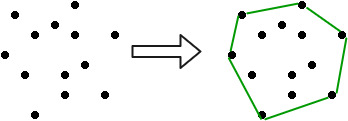
Input is an array of points specified by their x and y coordinates. The output is the convex hull of this set of points. Examples:
Input : points[] = {(0, 0), (0, 4), (-4, 0), (5, 0),
                   (0, -6), (1, 0)};
Output : (-4, 0), (5, 0), (0, -6), (0, 4)
Pre-requisite: Tangents between two convex polygons Algorithm: Given the set of points for which we have to find the convex hull. Suppose we know the convex hull of the left half points and the right half points, then the problem now is to merge these two convex hulls and determine the convex hull for the complete set. This can be done by finding the upper and lower tangent to the right and left convex hulls. This is illustrated here Tangents between two convex polygons Let the left convex hull be a and the right convex hull be b. Then the lower and upper tangents are named as 1 and 2 respectively, as shown in the figure. Then the red outline shows the final convex hull.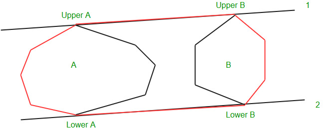 Now the problem remains, how to find the convex hull for the left and right half. Now recursion comes into the picture, we divide the set of points until the number of points in the set is very small, say 5, and we can find the convex hull for these points by the brute algorithm. The merging of these halves would result in the convex hull for the complete set of points. Note: We have used the brute algorithm to find the convex hull for a small number of points and it has a time complexity of
  . But some people suggest the following, the convex hull for 3 or fewer points is the complete set of points. This is correct but the problem comes when we try to merge a left convex hull of 2 points and right convex hull of 3 points, then the program gets trapped in an infinite loop in some special cases. So, to get rid of this problem I directly found the convex hull for 5 or fewer points by algorithm, which is somewhat greater but does not affect the overall complexity of the algorithm.
// A divide and conquer program to find convex
// hull of a given set of points.
#include<bits/stdc++.h>
using namespace std;
// stores the centre of polygon (It is made
// global because it is used in compare function)
pair<int, int> mid;
// determines the quadrant of a point
// (used in compare())
int quad(pair<int, int> p)
{
if (p.first >= 0 && p.second >= 0)
return 1;
if (p.first <= 0 && p.second >= 0)
return 2;
if (p.first <= 0 && p.second <= 0)
return 3;
return 4;
}
// Checks whether the line is crossing the polygon
int orientation(pair<int, int> a, pair<int, int> b,
pair<int, int> c)
{
int res = (b.second-a.second)*(c.first-b.first) -
(c.second-b.second)*(b.first-a.first);
if (res == 0)
return 0;
if (res > 0)
return 1;
return -1;
}
// compare function for sorting
bool compare(pair<int, int> p1, pair<int, int> q1)
{
pair<int, int> p = make_pair(p1.first - mid.first,
p1.second - mid.second);
pair<int, int> q = make_pair(q1.first - mid.first,
q1.second - mid.second);
int one = quad(p);
int two = quad(q);
if (one != two)
return (one < two);
return (p.second*q.first < q.second*p.first);
}
// Finds upper tangent of two polygons 'a' and 'b'
// represented as two vectors.
vector<pair<int, int>> merger(vector<pair<int, int> > a,
vector<pair<int, int> > b)
{
// n1 -> number of points in polygon a
// n2 -> number of points in polygon b
int n1 = a.size(), n2 = b.size();
int ia = 0, ib = 0;
for (int i=1; i<n1; i++)
if (a[i].first > a[ia].first)
ia = i;
// ib -> leftmost point of b
for (int i=1; i<n2; i++)
if (b[i].first < b[ib].first)
ib=i;
// finding the upper tangent
int inda = ia, indb = ib;
bool done = 0;
while (!done)
{
done = 1;
while (orientation(b[indb], a[inda], a[(inda+1)%n1]) >=0)
inda = (inda + 1) % n1;
while (orientation(a[inda], b[indb], b[(n2+indb-1)%n2]) <=0)
{
indb = (n2+indb-1)%n2;
done = 0;
}
}
int uppera = inda, upperb = indb;
inda = ia, indb=ib;
done = 0;
int g = 0;
while (!done)//finding the lower tangent
{
done = 1;
while (orientation(a[inda], b[indb], b[(indb+1)%n2])>=0)
indb=(indb+1)%n2;
while (orientation(b[indb], a[inda], a[(n1+inda-1)%n1])<=0)
{
inda=(n1+inda-1)%n1;
done=0;
}
}
int lowera = inda, lowerb = indb;
vector<pair<int, int>> ret;
//ret contains the convex hull after merging the two convex hulls
//with the points sorted in anti-clockwise order
int ind = uppera;
ret.push_back(a[uppera]);
while (ind != lowera)
{
ind = (ind+1)%n1;
ret.push_back(a[ind]);
}
ind = lowerb;
ret.push_back(b[lowerb]);
while (ind != upperb)
{
ind = (ind+1)%n2;
ret.push_back(b[ind]);
}
return ret;
}
// Brute force algorithm to find convex hull for a set
// of less than 6 points
vector<pair<int, int>> bruteHull(vector<pair<int, int>> a)
{
// Take any pair of points from the set and check
// whether it is the edge of the convex hull or not.
// if all the remaining points are on the same side
// of the line then the line is the edge of convex
// hull otherwise not
set<pair<int, int> >s;
for (int i=0; i<a.size(); i++)
{
for (int j=i+1; j<a.size(); j++)
{
int x1 = a[i].first, x2 = a[j].first;
int y1 = a[i].second, y2 = a[j].second;
int a1 = y1-y2;
int b1 = x2-x1;
int c1 = x1*y2-y1*x2;
int pos = 0, neg = 0;
for (int k=0; k<a.size(); k++)
{
if (a1*a[k].first+b1*a[k].second+c1 <= 0)
neg++;
if (a1*a[k].first+b1*a[k].second+c1 >= 0)
pos++;
}
if (pos == a.size() || neg == a.size())
{
s.insert(a[i]);
s.insert(a[j]);
}
}
}
vector<pair<int, int>>ret;
for (auto e:s)
ret.push_back(e);
// Sorting the points in the anti-clockwise order
mid = {0, 0};
int n = ret.size();
for (int i=0; i<n; i++)
{
mid.first += ret[i].first;
mid.second += ret[i].second;
ret[i].first *= n;
ret[i].second *= n;
}
sort(ret.begin(), ret.end(), compare);
for (int i=0; i<n; i++)
ret[i] = make_pair(ret[i].first/n, ret[i].second/n);
return ret;
}
// Returns the convex hull for the given set of points
vector<pair<int, int>> divide(vector<pair<int, int>> a)
{
// If the number of points is less than 6 then the
// function uses the brute algorithm to find the
// convex hull
if (a.size() <= 5)
return bruteHull(a);
// left contains the left half points
// right contains the right half points
vector<pair<int, int>>left, right;
for (int i=0; i<a.size()/2; i++)
left.push_back(a[i]);
for (int i=a.size()/2; i<a.size(); i++)
right.push_back(a[i]);
// convex hull for the left and right sets
vector<pair<int, int>>left_hull = divide(left);
vector<pair<int, int>>right_hull = divide(right);
// merging the convex hulls
return merger(left_hull, right_hull);
}
// Driver code
int main()
{
vector<pair<int, int> > a;
a.push_back(make_pair(0, 0));
a.push_back(make_pair(1, -4));
a.push_back(make_pair(-1, -5));
a.push_back(make_pair(-5, -3));
a.push_back(make_pair(-3, -1));
a.push_back(make_pair(-1, -3));
a.push_back(make_pair(-2, -2));
a.push_back(make_pair(-1, -1));
a.push_back(make_pair(-2, -1));
a.push_back(make_pair(-1, 1));
int n = a.size();
// sorting the set of points according
// to the x-coordinate
sort(a.begin(), a.end());
vector<pair<int, int> >ans = divide(a);
cout << "convex hull:\n";
for (auto e:ans)
cout << e.first << " "
<< e.second << endl;
return 0;
}
convex hull:
-5 -3
-1 -5
1 -4
0 0
-1 1
0/1 kanpsack problem
/* A Naive recursive implementation of
0-1 Knapsack problem */
#include <bits/stdc++.h>
using namespace std;

// A utility function that returns
// maximum of two integers
int max(int a, int b) { return (a > b) ? a : b; }

// Returns the maximum value that
// can be put in a knapsack of capacity W
int knapSack(int W, int wt[], int val[], int n)
{

	// Base Case
	if (n == 0 || W == 0)
		return 0;

	// If weight of the nth item is more
	// than Knapsack capacity W, then
	// this item cannot be included
	// in the optimal solution
	if (wt[n - 1] > W)
		return knapSack(W, wt, val, n - 1);

	// Return the maximum of two cases:
	// (1) nth item included
	// (2) not included
	else
		return max(
			val[n - 1]
				+ knapSack(W - wt[n - 1], wt, val, n - 1),
			knapSack(W, wt, val, n - 1));
}

// Driver code
int main()
{
	int profit[] = { 60, 100, 120 };
	int weight[] = { 10, 20, 30 };
	int W = 50;
	int n = sizeof(profit) / sizeof(profit[0]);
	cout << knapSack(W, weight, profit, n);
	return 0;
}

// This code is contributed by rathbhupendra
Wonderfull Blog Article. Thank you so much for sharing.
ReplyDeleteAzure Databricks Training
Azure Data Engineering Training
Azure Data Engineering Online Training
Data Engineering Training Hyderabad
Azure Data Engineering Training Hyderabad
Microsoft Power BI Training
Power BI Online Training
NicNice article. Please check office workstations for best deal.
ReplyDeleteGood Blog Article.Thanks for sharing.
ReplyDeleteData Analytics Training
Data Analytics Online Training
Data Analytics Course in Hyderabad
Data Analytics Training in Ameerpet
Data Analytics Training in Hyderabad
Data Analysis Online Training Course
Data Analytics Online Training Institute
Data Analytics Course
Data Analysis Online Course
Nice Blog Article.Thanks for sharing the information.
ReplyDeleteGenerative AI (GenAI) Courses Online
Generative AI Course Training in Hyderabad
DataScience with Generative AI Course
Gen AI Course in Hyderabad
Generative AI Training in Ameerpet
DataScience Training Institute in Hyderabad
AI and ML Training in Hyderabad
DataScience Course in Hyderabad
Generative AI Online Training Courses
Your writing changed my life in a lot more positive way. Many thanks.
ReplyDeleteHire Java Developer in Chennai